Visualization tutorial

This tutorial show the visualization process of our processed Stereo-seq mosue midbrain dataset

• The command for running on this dataset is:

ONTraC \
    --meta-input data/stereo_seq_brain/original_data.csv \
    --NN-dir output/stereo_seq_NN \
    --GNN-dir output/stereo_seq_GNN \
    --NT-dir output/stereo_seq_NT \
    --device cuda \
    -s 42 \
    --lr 0.03 \
    --hidden-feats 4 \
    -k 6 \
    --modularity-loss-weight 0.3 \
    --regularization-loss-weight 0.1 \
    --purity-loss-weight 300 \
    --beta 0.03 2>&1 | tee log/stereo_seq.log

Note

The input dataset and output files could be downloaded from our Zenodo repository.

Preparation

Install Required Packages

pip install "ONTraC[analysis]"

Load Dataset

import requests

# URL of the file
url = "https://zenodo.org/records/15571644/files/Stereo_seq_data.zip"

# Local file path to save the file
file_path = "./Stereo_seq_data.zip"

try:
    # Send a GET request to the URL
    response = requests.get(url)
    response.raise_for_status()  # Check if the request was successful

    # Write the content to the file
    with open(file_path, "wb") as file:
        file.write(response.content)

    print(f"File downloaded and saved to {file_path}")
except requests.exceptions.RequestException as e:
    print(f"An error occurred: {e}")

File downloaded and saved to ./Stereo_seq_data.zip

import zipfile

# Path to the zip file
zip_file_path = "Stereo_seq_data.zip"

# Directory where files will be extracted
extract_to_path = "./"

try:
    # Open the zip file
    with zipfile.ZipFile(zip_file_path, 'r') as zip_ref:
        # Extract all files to the specified directory
        zip_ref.extractall(extract_to_path)

    print(f"Files extracted to '{extract_to_path}'")
except zipfile.BadZipFile:
    print("The file is not a valid zip file.")

Files extracted to './'

Visualization through Command Line

ONTraC_analysis \
    -o analysis_output/stereo_seq \
    -l Stereo_seq_data/ONTraC_run_log/stereo_midbrain_base.log \
    --NN-dir Stereo_seq_data/ONTraC_output/stereo_midbrain_base_NN \
    --GNN-dir Stereo_seq_data/ONTraC_output/stereo_midbrain_base_GNN \
    --NT-dir Stereo_seq_data/ONTraC_output/stereo_midbrain_base_NT \
    -r

Visualization Step-by-step

If you want to adjust the figures, here is the example codes for step-by-step analysis using Python. We recommand you using jupyter notebook or jupyter lab here.

Load Modules

import matplotlib as mpl

mpl.rcParams['pdf.fonttype'] = 42
mpl.rcParams['ps.fonttype'] = 42
mpl.rcParams['font.family'] = 'Arial'
import matplotlib.pyplot as plt
import seaborn as sns

from ONTraC.analysis.data import AnaData

Plotting Preparation

from optparse import Values

options = Values()
options.NN_dir = 'Stereo_seq_data/ONTraC_output/stereo_midbrain_base_NN'
options.GNN_dir = 'Stereo_seq_data/ONTraC_output/stereo_midbrain_base_GNN'
options.NT_dir = 'Stereo_seq_data/ONTraC_output/stereo_midbrain_base_NT'
options.log = 'Stereo_seq_data/ONTraC_run_log/stereo_midbrain_base.log'
options.reverse = True  # Set it to False if you don't want reverse NT score
options.output = None  # We save the output figure by our self here
ana_data = AnaData(options)

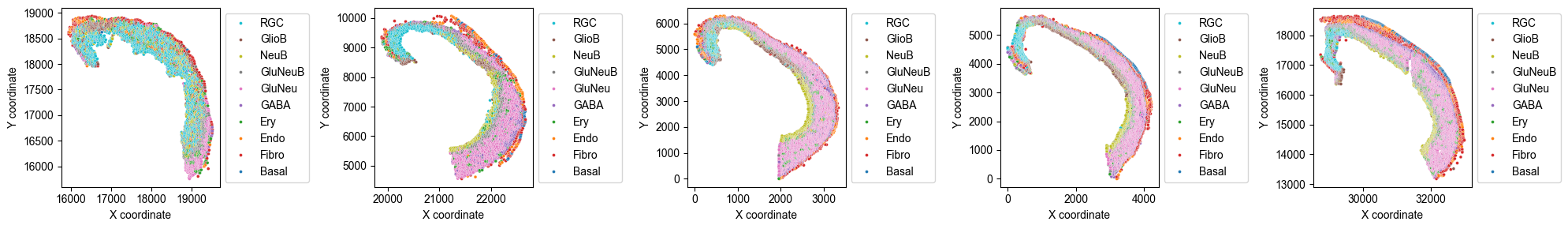
Spatial Cell Type Distribution

from ONTraC.analysis.cell_type import plot_spatial_cell_type_distribution_dataset_from_anadata

fig, axes = plot_spatial_cell_type_distribution_dataset_from_anadata(ana_data = ana_data,
                                                                     hue_order = ['RGC', 'GlioB', 'NeuB', 'GluNeuB', 'GluNeu', 'GABA', 'Ery', 'Endo', 'Fibro', 'Basal'])

for ax in axes:
    # ax.set_aspect('equal', 'box')  # uncomment this line if you want set the x and y axis with same scaling
    # ax.set_xticks([])  # uncomment this line if you don't want to show x coordinates
    # ax.set_yticks([]) # uncomment this line if you don't want to show y coordinates
    pass

fig.tight_layout()
# fig.savefig('figures/Spatial_cell_type.png', dpi=150)  # uncomment this line if you want save the results

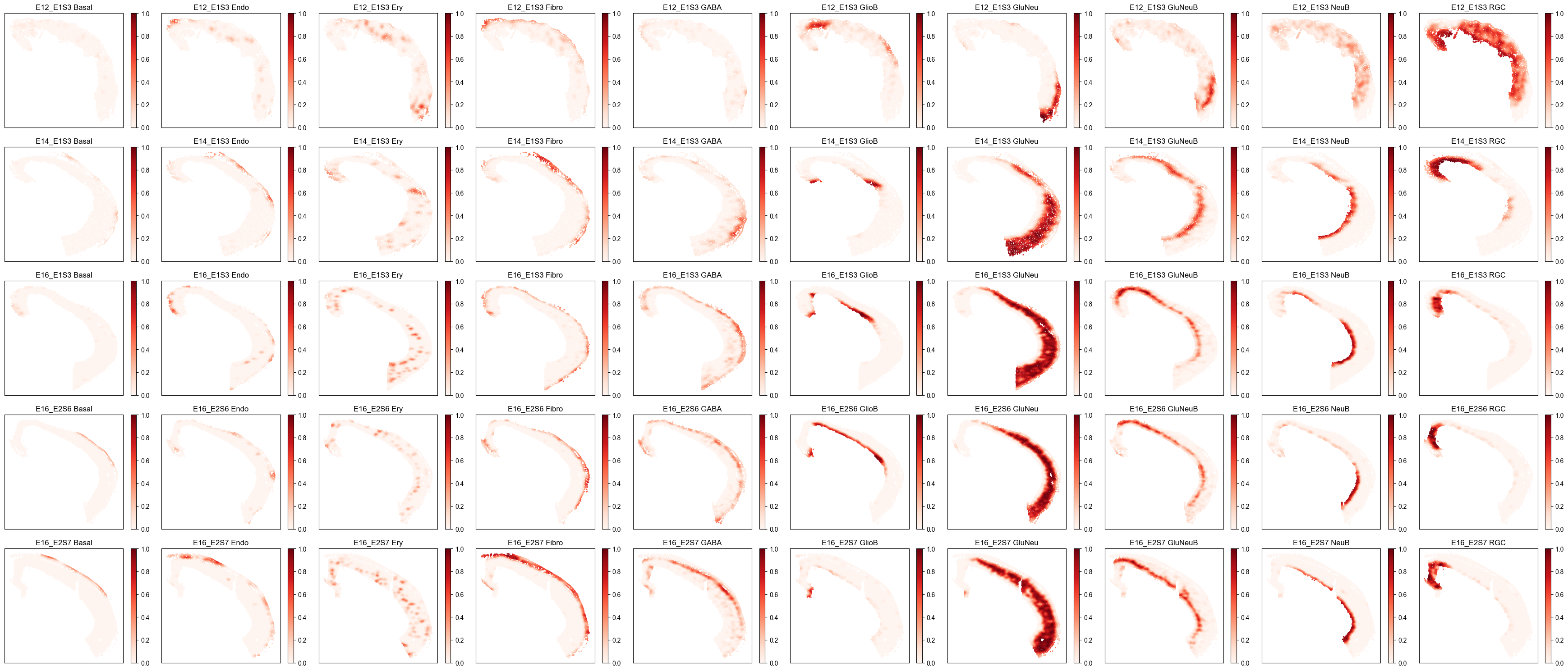
Spatial Cell Type Composition Distribution

from ONTraC.analysis.spatial import plot_cell_type_composition_dataset_from_anadata

fig, axes = plot_cell_type_composition_dataset_from_anadata(ana_data=ana_data)
# fig.savefig('figures/cell_type_compostion.png', dpi=100)  # uncomment this line if you want save the results

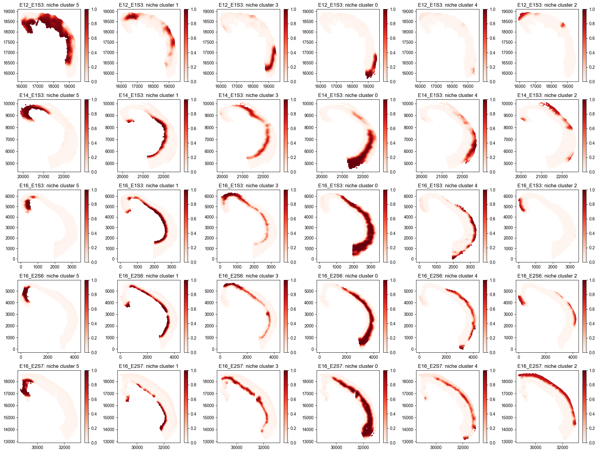
Niche Cluster

Spatial Niche Cluster Loadings Distribution

from ONTraC.analysis.niche_cluster import plot_niche_cluster_loadings_dataset_from_anadata

fig, axes = plot_niche_cluster_loadings_dataset_from_anadata(ana_data=ana_data)
# fig.savefig('figures/Spatial_niche_clustering_loadings.png', dpi=100)  # uncomment this line if you want save the results

Niche Cluster Connectivity

from ONTraC.analysis.niche_cluster import plot_niche_cluster_connectivity_from_anadata

fig, axes = plot_niche_cluster_connectivity_from_anadata(ana_data=ana_data)
# fig.savefig('figures/Niche_cluster_connectivity.png', dpi=300)  # uncomment this line if you want save the results

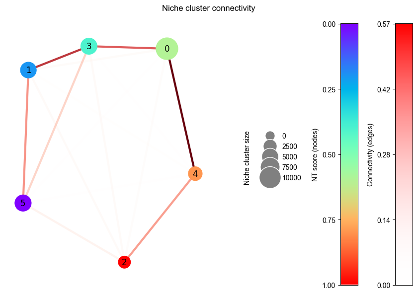
Note

This figure show the spatial connectivity between each niche cluster which will be used for niche trajectory construction.

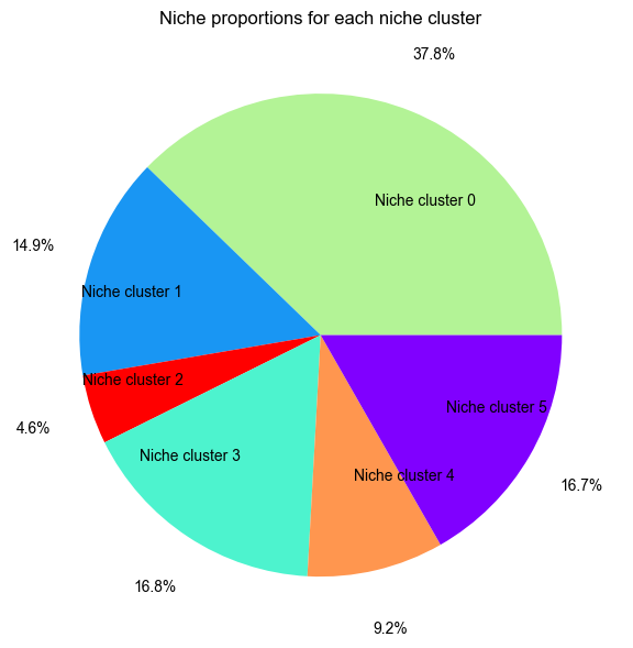
Niche Cluster Proportion

from ONTraC.analysis.niche_cluster import plot_cluster_proportion_from_anadata

fig, ax = plot_cluster_proportion_from_anadata(ana_data=ana_data)
# fig.savefig('figures/Niche_cluster_proportions.png', dpi=300)  # uncomment this line if you want save the results

Cell Type X Niche Cluster

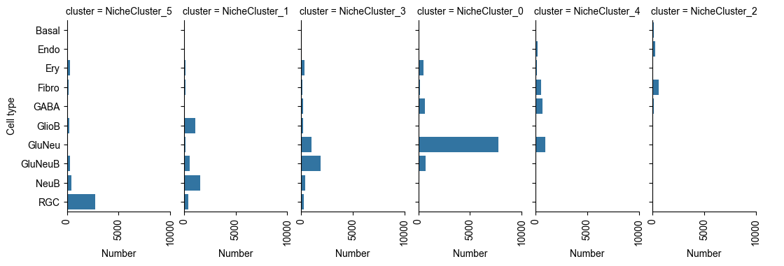
Number of Cells of Each Cell Type in Each Niche Cluster

from ONTraC.analysis.cell_type import plot_cell_type_loading_in_niche_clusters_from_anadata

g = plot_cell_type_loading_in_niche_clusters_from_anadata(ana_data=ana_data)
# g.savefig('figures/cell_type_loading_in_niche_clusters.png', dpi=300)  # uncomment this line if you want save the results

Cell Type Composition Normalized by Each Niche Cluster

from ONTraC.analysis.cell_type import plot_cell_type_com_in_niche_clusters_from_anadata

fig, ax = plot_cell_type_com_in_niche_clusters_from_anadata(ana_data=ana_data)
# fig.savefig('figures/cell_type_composition_in_niche_clusters.png', dpi=300)  # uncomment this line if you want save the results

Note

This heatmap show the cell type composition within each niche cluster. Sum of each row equals to 1.

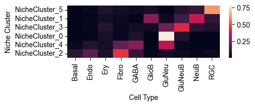
Cell Type Composition Normalized by Each Cell Type

from ONTraC.analysis.cell_type import plot_cell_type_dis_across_niche_cluster_from_anadata

fig, ax = plot_cell_type_dis_across_niche_cluster_from_anadata(ana_data=ana_data)
# fig.savefig('figures/cell_type_dis_across_niche_cluster.png', dpi=300)  # uncomment this line if you want save the results

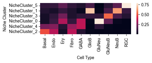
Note

This heatmap show the cell type distribution across niche clusters. Sum of each column equals to 1.

Spatial Niche-level NT Score Distribution

from ONTraC.analysis.spatial import plot_niche_NT_score_dataset_from_anadata

fig, ax = plot_niche_NT_score_dataset_from_anadata(ana_data=ana_data)
# fig.savefig('figures/niche_NT_score.png', dpi=200)  # uncomment this line if you want save the results

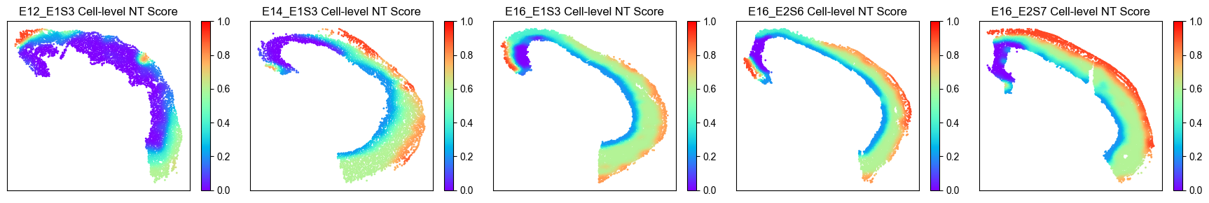
Spatial Cell-level NT Score Distribution

from ONTraC.analysis.spatial import plot_cell_NT_score_dataset_from_anadata

fig, ax = plot_cell_NT_score_dataset_from_anadata(ana_data=ana_data)
# fig.savefig('figures/cell_NT_score.png', dpi=200)  # uncomment this line if you want save the results

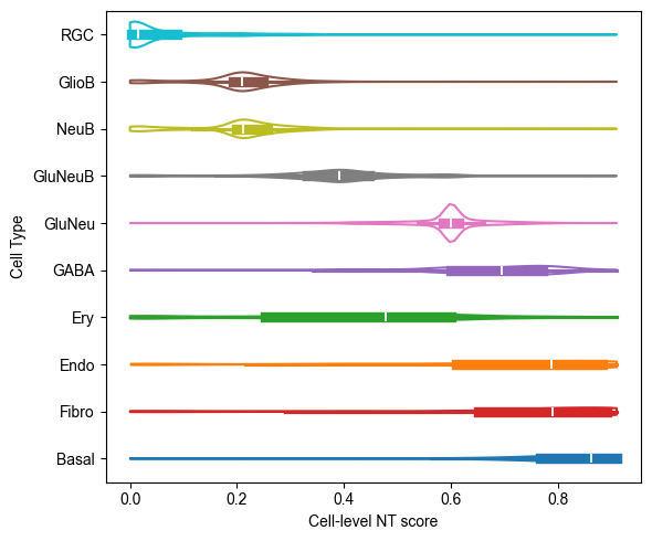
Cell-level NT Score Distribution for Each Cell Type

from ONTraC.analysis.cell_type import plot_violin_cell_type_along_NT_score_from_anadata

fig, ax = plot_violin_cell_type_along_NT_score_from_anadata(ana_data=ana_data,
                                                            order=['RGC', 'GlioB', 'NeuB', 'GluNeuB', 'GluNeu', 'GABA', 'Ery', 'Endo', 'Fibro', 'Basal'],  # change based on your own dataset or remove this line
                                                           )
# fig.savefig('figures/cell_type_along_NT_score_violin.png', dpi=300)  # uncomment this line if you want save the results