Spatial trajectory-based analysis

This tutorial demonstrates how to analyze feature changes along the trajectory inferred by ONTraC.

Features may include cell type composition, gene expression, regulon activity, or any other cell-level or niche-level scores.

Load Modules

import numpy as np
import pandas as pd
import matplotlib as mpl
mpl.rcParams['pdf.fonttype'] = 42
mpl.rcParams['ps.fonttype'] = 42
mpl.rcParams['font.sans-serif'] = 'Arial'
import matplotlib.pyplot as plt
import seaborn as sns
from pprint import pprint
%matplotlib inline

from optparse import Values

from ONTraC.analysis.data import AnaData
from ONTraC.utils import write_version_info

write_version_info()

##################################################################################

         ▄▄█▀▀██   ▀█▄   ▀█▀ █▀▀██▀▀█                   ▄▄█▀▀▀▄█
        ▄█▀    ██   █▀█   █     ██    ▄▄▄ ▄▄   ▄▄▄▄   ▄█▀     ▀
        ██      ██  █ ▀█▄ █     ██     ██▀ ▀▀ ▀▀ ▄██  ██
        ▀█▄     ██  █   ███     ██     ██     ▄█▀ ██  ▀█▄      ▄
         ▀▀█▄▄▄█▀  ▄█▄   ▀█    ▄██▄   ▄██▄    ▀█▄▄▀█▀  ▀▀█▄▄▄▄▀

                        version: 1.2.2

##################################################################################

from ONTraC.analysis.trajectory import (construct_meta_cell_along_trajectory,
                                        cal_features_correlation_along_trajectory,
                                        plot_scatter_feat_along_trajectory,
                                        plot_cell_type_composition_along_trajectory_from_anadata,
                                        plot_cell_type_composition_along_trajectory)

from scipy import stats
from statsmodels.stats.multitest import multipletests

import gseapy as gp

Dataset Explanation

The Stereo-seq mouse embryonic midbrain dataset was originally published by Chen, et al. The raw data could be download from the MOSTA website.

We assume that you have runned ONTraC on Stereo-seq mouse embryonic midbrain dataset according to our example tutorial.

Load Data

Download dataset

import requests

# URL of the file
url = "https://zenodo.org/records/15571644/files/Stereo_seq_data.zip"

# Local file path to save the file
file_path = "./Stereo_seq_data.zip"

try:
    # Send a GET request to the URL
    response = requests.get(url)
    response.raise_for_status()  # Check if the request was successful

    # Write the content to the file
    with open(file_path, "wb") as file:
        file.write(response.content)

    print(f"File downloaded and saved to {file_path}")
except requests.exceptions.RequestException as e:
    print(f"An error occurred: {e}")

File downloaded and saved to ./Stereo_seq_data.zip

import zipfile

# Path to the zip file
zip_file_path = "Stereo_seq_data.zip"

# Directory where files will be extracted
extract_to_path = "./"

try:
    # Open the zip file
    with zipfile.ZipFile(zip_file_path, 'r') as zip_ref:
        # Extract all files to the specified directory
        zip_ref.extractall(extract_to_path)

    print(f"Files extracted to '{extract_to_path}'")
except zipfile.BadZipFile:
    print("The file is not a valid zip file.")

Files extracted to './'

ONTraC output

vis_options = Values()
vis_options.NN_dir = './Stereo_seq_data/ONTraC_output/stereo_midbrain_base_NN/'
vis_options.GNN_dir = './Stereo_seq_data/ONTraC_output/stereo_midbrain_base_GNN/'
vis_options.NT_dir = './Stereo_seq_data/ONTraC_output/stereo_midbrain_base_NT/'
vis_options.reverse = True
vis_options.output = None

ana_data = AnaData(vis_options)

ana_data.meta_data_df.head()

	Sample	Cell_Type	x	y
Cell_ID
E12_E1S3_100034	E12_E1S3	Fibro	15940.0	18584.0
E12_E1S3_100035	E12_E1S3	Fibro	15942.0	18623.0
E12_E1S3_100191	E12_E1S3	Endo	15965.0	18619.0
E12_E1S3_100256	E12_E1S3	Fibro	15969.0	18717.0
E12_E1S3_100264	E12_E1S3	Fibro	15974.0	18692.0

Differentiation potency

The differentialtion potency was calculated using moscot.

Please refer our processing codes for details.

ot_res1 = pd.read_csv('./Stereo_seq_data/source/moscot/E14_E16_1_cm.csv.gz', index_col=0)
temp = pd.read_csv('./Stereo_seq_data/source/moscot/ss0_E14_E1S3_loc.csv.gz',index_col = 0)
ot_res1.index = temp.index
temp = pd.read_csv('./Stereo_seq_data/source/moscot/ss0_E16_E1S3_loc.csv.gz',index_col = 0)
ot_res1.columns = temp.index
ot_res1.head()

	E16_E1S3_21	E16_E1S3_22	E16_E1S3_23	E16_E1S3_26	E16_E1S3_27	E16_E1S3_28	E16_E1S3_29	E16_E1S3_31	E16_E1S3_32	E16_E1S3_33	...	E16_E1S3_6920	E16_E1S3_6921	E16_E1S3_6923	E16_E1S3_6924	E16_E1S3_6925	E16_E1S3_6926	E16_E1S3_6928	E16_E1S3_6929	E16_E1S3_6930	E16_E1S3_6931
E14_E1S3_170808	0.0	0.0	0.0	0.0	0.0	0.0	0.0	0.0	0.0	0.0	...	0.000000e+00	0.0	0.000000	0.0	0.0	0.0	0.000000e+00	0.0	0.0	0.000000e+00
E14_E1S3_170916	0.0	0.0	0.0	0.0	0.0	0.0	0.0	0.0	0.0	0.0	...	6.345486e-31	0.0	0.000154	0.0	0.0	0.0	0.000000e+00	0.0	0.0	4.531762e-26
E14_E1S3_170934	0.0	0.0	0.0	0.0	0.0	0.0	0.0	0.0	0.0	0.0	...	0.000000e+00	0.0	0.000000	0.0	0.0	0.0	2.703351e-37	0.0	0.0	0.000000e+00
E14_E1S3_171016	0.0	0.0	0.0	0.0	0.0	0.0	0.0	0.0	0.0	0.0	...	0.000000e+00	0.0	0.000000	0.0	0.0	0.0	0.000000e+00	0.0	0.0	0.000000e+00
E14_E1S3_171024	0.0	0.0	0.0	0.0	0.0	0.0	0.0	0.0	0.0	0.0	...	0.000000e+00	0.0	0.000000	0.0	0.0	0.0	0.000000e+00	0.0	0.0	0.000000e+00

5 rows × 6643 columns

ot_res2 = pd.read_csv('./Stereo_seq_data/source/moscot/E14_E16_2_cm.csv.gz', index_col=0)
temp = pd.read_csv('./Stereo_seq_data/source/moscot/ss0_E14_E1S3_loc.csv.gz',index_col = 0)
ot_res2.index = temp.index
temp = pd.read_csv('./Stereo_seq_data/source/moscot/ss0_E16_E2S6_loc.csv.gz',index_col = 0)
ot_res2.columns = temp.index
ot_res2.head()

	E16_E2S6_119	E16_E2S6_147	E16_E2S6_164	E16_E2S6_193	E16_E2S6_199	E16_E2S6_203	E16_E2S6_217	E16_E2S6_222	E16_E2S6_230	E16_E2S6_234	...	E16_E2S6_36290	E16_E2S6_36348	E16_E2S6_36407	E16_E2S6_36523	E16_E2S6_36607	E16_E2S6_36632	E16_E2S6_36755	E16_E2S6_36782	E16_E2S6_36838	E16_E2S6_36891
E14_E1S3_170808	0.0	0.0	0.0	0.0	0.0	0.0	0.0	0.0	0.0	0.0	...	0.0	0.000000	0.000000	0.000000e+00	0.0	0.0	0.000000e+00	0.0	0.0	0.0
E14_E1S3_170916	0.0	0.0	0.0	0.0	0.0	0.0	0.0	0.0	0.0	0.0	...	0.0	0.000000	0.000000	0.000000e+00	0.0	0.0	0.000000e+00	0.0	0.0	0.0
E14_E1S3_170934	0.0	0.0	0.0	0.0	0.0	0.0	0.0	0.0	0.0	0.0	...	0.0	0.000112	0.000002	9.689674e-31	0.0	0.0	8.916933e-08	0.0	0.0	0.0
E14_E1S3_171016	0.0	0.0	0.0	0.0	0.0	0.0	0.0	0.0	0.0	0.0	...	0.0	0.000000	0.000000	0.000000e+00	0.0	0.0	1.239693e-06	0.0	0.0	0.0
E14_E1S3_171024	0.0	0.0	0.0	0.0	0.0	0.0	0.0	0.0	0.0	0.0	...	0.0	0.000000	0.000000	0.000000e+00	0.0	0.0	0.000000e+00	0.0	0.0	0.0

5 rows × 5506 columns

ot_res3 = pd.read_csv('./Stereo_seq_data/source/moscot/E14_E16_3_cm.csv.gz', index_col=0)
temp = pd.read_csv('./Stereo_seq_data/source/moscot/ss0_E14_E1S3_loc.csv.gz',index_col = 0)
ot_res3.index = temp.index
temp = pd.read_csv('./Stereo_seq_data/source/moscot/ss0_E16_E2S7_loc.csv.gz',index_col = 0)
ot_res3.columns = temp.index
ot_res3.head()

	E16_E2S7_291152	E16_E2S7_291165	E16_E2S7_291300	E16_E2S7_291398	E16_E2S7_291435	E16_E2S7_291487	E16_E2S7_291503	E16_E2S7_291550	E16_E2S7_291585	E16_E2S7_291591	...	E16_E2S7_326320	E16_E2S7_326323	E16_E2S7_326324	E16_E2S7_326325	E16_E2S7_326329	E16_E2S7_326357	E16_E2S7_326359	E16_E2S7_326384	E16_E2S7_326391	E16_E2S7_326412
E14_E1S3_170808	0.0	1.598103e-18	0.0	0.0	7.107961e-09	0.0	1.541208e-25	0.0	0.0	0.0	...	0.0	0.0	0.0	0.0	0.0	0.0	0.0	0.0	0.0	0.0
E14_E1S3_170916	0.0	0.000000e+00	0.0	0.0	0.000000e+00	0.0	0.000000e+00	0.0	0.0	0.0	...	0.0	0.0	0.0	0.0	0.0	0.0	0.0	0.0	0.0	0.0
E14_E1S3_170934	0.0	0.000000e+00	0.0	0.0	0.000000e+00	0.0	0.000000e+00	0.0	0.0	0.0	...	0.0	0.0	0.0	0.0	0.0	0.0	0.0	0.0	0.0	0.0
E14_E1S3_171016	0.0	0.000000e+00	0.0	0.0	0.000000e+00	0.0	0.000000e+00	0.0	0.0	0.0	...	0.0	0.0	0.0	0.0	0.0	0.0	0.0	0.0	0.0	0.0
E14_E1S3_171024	0.0	0.000000e+00	0.0	0.0	0.000000e+00	0.0	0.000000e+00	0.0	0.0	0.0	...	0.0	0.0	0.0	0.0	0.0	0.0	0.0	0.0	0.0	0.0

5 rows × 7261 columns

Gene expression

E14_RGC_scaled_exp = pd.read_csv('./Stereo_seq_data/source/stereo_seq_E14_RGC_scaled_exp.csv.gz', index_col=0)
E14_RGC_scaled_exp.head()

	0610005C13Rik	0610006L08Rik	0610009B22Rik	0610009O20Rik	0610010F05Rik	0610010K14Rik	0610012G03Rik	0610025J13Rik	0610030E20Rik	0610031O16Rik	...	Zw10	Zwilch	Zwint	Zxdb	Zxdc	Zyg11a	Zyg11b	Zyx	Zzef1	Zzz3
Cell_ID
E14_E1S3_171289	-0.036511	-0.008535	-0.198124	-0.106792	-0.239179	3.277203	-0.321011	-0.025192	-0.088172	-0.008486	...	-0.091104	-0.068489	-0.389927	-0.073764	-0.117644	-0.043855	-0.223836	-0.21233	-0.148131	-0.199425
E14_E1S3_171863	-0.036511	-0.008535	-0.198124	-0.106792	-0.239179	-0.307818	-0.321011	-0.025192	-0.088172	-0.008486	...	-0.091104	-0.068489	-0.389927	-0.073764	9.345431	-0.043855	-0.223836	-0.21233	-0.148131	-0.199425
E14_E1S3_171967	-0.036511	-0.008535	-0.198124	-0.106792	-0.239179	-0.307818	-0.321011	-0.025192	-0.088172	-0.008486	...	-0.091104	-0.068489	-0.389927	-0.073764	-0.117644	-0.043855	-0.223836	-0.21233	-0.148131	-0.199425
E14_E1S3_171983	-0.036511	-0.008535	-0.198124	-0.106792	-0.239179	2.074143	-0.321011	-0.025192	-0.088172	-0.008486	...	-0.091104	-0.068489	-0.389927	-0.073764	-0.117644	-0.043855	-0.223836	-0.21233	-0.148131	-0.199425
E14_E1S3_172013	-0.036511	-0.008535	-0.198124	-0.106792	-0.239179	-0.307818	-0.321011	-0.025192	-0.088172	-0.008486	...	-0.091104	-0.068489	-0.389927	-0.073764	-0.117644	-0.043855	-0.223836	-0.21233	-0.148131	-0.199425

5 rows × 23944 columns

Regulon activities

Regulon activities were calculated using pySCENIC.

Please refer our processing codes for details.

regulon_aucell_df = pd.read_csv('./Stereo_seq_data/source/stereo_seq.auc.csv.gz', index_col=0)
regulon_aucell_df.head()

	Ahr	Alx1	Alx3	Alx4	Ar	Arid3a	Arntl2	Arx	Atf1	Atf3	...	Zfp821	Zfp874b	Zfp941	Zfp944	Zfp979	Zic1	Zkscan14	Zkscan16	Zscan20	Zxdc
Cell
E12_E1S3_100034	0.0	0.014262	0.009032	0.038966	0.0	0.001760	0.0	0.000000	0.0	0.134952	...	0.0	0.000000	0.0	0.0	0.0	0.051056	0.045712	0.017288	0.0	0.0
E12_E1S3_100035	0.0	0.017741	0.017087	0.000000	0.0	0.003681	0.0	0.000000	0.0	0.167847	...	0.0	0.003940	0.0	0.0	0.0	0.064695	0.062440	0.026075	0.0	0.0
E12_E1S3_100191	0.0	0.009400	0.009933	0.026062	0.0	0.001426	0.0	0.000000	0.0	0.129891	...	0.0	0.000000	0.0	0.0	0.0	0.088422	0.042828	0.015757	0.0	0.0
E12_E1S3_100256	0.0	0.017928	0.017399	0.000000	0.0	0.003750	0.0	0.000000	0.0	0.168128	...	0.0	0.004096	0.0	0.0	0.0	0.048256	0.062728	0.091552	0.0	0.0
E12_E1S3_100264	0.0	0.019671	0.019565	0.042947	0.0	0.004231	0.0	0.080958	0.0	0.176000	...	0.0	0.005547	0.0	0.0	0.0	0.049611	0.066910	0.028448	0.0	0.0

5 rows × 304 columns

Msigdb gene sets

Please refer release note for details.

import requests

# URL of the file
url = "https://data.broadinstitute.org/gsea-msigdb/msigdb/release/7.5.1/c5.go.bp.v7.5.1.symbols.gmt"

# Local file path to save the file
file_path = "./c5.go.bp.v7.5.1.symbols.gmt"

try:
    # Send a GET request to the URL
    response = requests.get(url)
    response.raise_for_status()  # Check if the request was successful

    # Write the content to the file
    with open(file_path, "wb") as file:
        file.write(response.content)

    print(f"File downloaded and saved to {file_path}")
except requests.exceptions.RequestException as e:
    print(f"An error occurred: {e}")

File downloaded and saved to ./c5.go.bp.v7.5.1.symbols.gmt

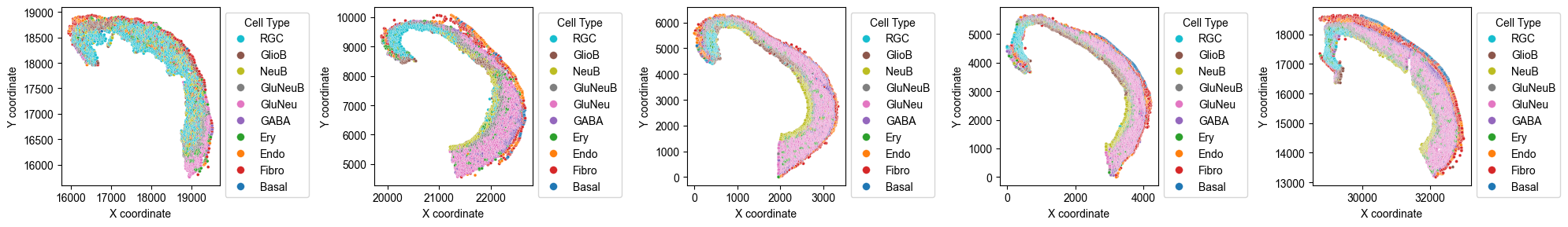
Dataset overview

from ONTraC.analysis.cell_type import plot_spatial_cell_type_distribution_dataset_from_anadata

fig, axes = plot_spatial_cell_type_distribution_dataset_from_anadata(ana_data = ana_data,
                                                                     hue_order = ['RGC', 'GlioB', 'NeuB', 'GluNeuB', 'GluNeu', 'GABA', 'Ery', 'Endo', 'Fibro', 'Basal'])

for ax in axes:
    ax.legend(title='Cell Type', loc='upper left', bbox_to_anchor=(1,1), markerscale=2.5)
    # ax.set_aspect('equal', 'box')  # uncomment this line if you want set the x and y axis with same scaling
    # ax.set_xticks([])  # uncomment this line if you don't want to show x coordinates
    # ax.set_yticks([])  # uncomment this line if you don't want to show y coordinates
    # ax.invert_xaxis()  # uncomment this line if you want to invert x axis
    # ax.invert_yaxis()  # uncomment this line if you want to invert y axis
    
    pass

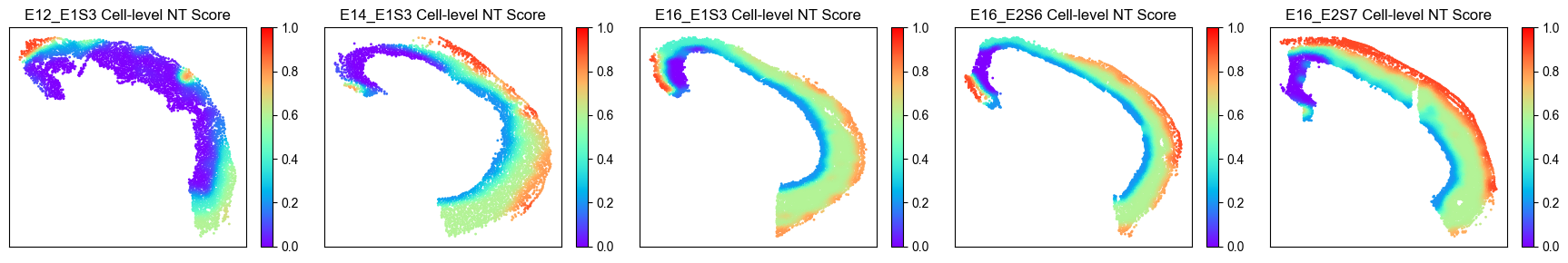
Spatial distribution of NT scores

We visualize the spatial distribution of NT scores for each cell to illustrate the spatial trajectory.

Spatial distribution of NT scores for all cells

from ONTraC.analysis.spatial import plot_cell_NT_score_dataset_from_anadata

fig, axes = plot_cell_NT_score_dataset_from_anadata(ana_data)

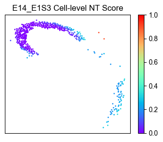
Spatial distribution of NT scores for E14.5 RGCs only

# Selecting E14.5 RGCs from the dataset
plot_meta_data = ana_data.meta_data_df[(ana_data.meta_data_df['Sample'] == 'E14_E1S3') & (ana_data.meta_data_df['Cell_Type'] == 'RGC')]
plot_meta_data.head()

	Sample	Cell_Type	x	y
Cell_ID
E14_E1S3_171289	E14_E1S3	RGC	19941.0	9116.0
E14_E1S3_171863	E14_E1S3	RGC	20024.0	9512.0
E14_E1S3_171967	E14_E1S3	RGC	20040.0	9397.0
E14_E1S3_171983	E14_E1S3	RGC	20040.0	9219.0
E14_E1S3_172013	E14_E1S3	RGC	20036.0	9352.0

plot_NT_score = ana_data.NT_score.loc[plot_meta_data.index]
plot_NT_score.head()

	x	y	Niche_NTScore	Cell_NTScore
Cell_ID
E14_E1S3_171289	19941.0	9116.0	0.862209	0.894205
E14_E1S3_171863	20024.0	9512.0	0.983229	0.979535
E14_E1S3_171967	20040.0	9397.0	0.994614	0.980553
E14_E1S3_171983	20040.0	9219.0	0.988135	0.958657
E14_E1S3_172013	20036.0	9352.0	0.994703	0.976718

# visualization

from ONTraC.analysis.spatial import plot_cell_NT_score_dataset

fig, ax = plot_cell_NT_score_dataset(meta_data_df=plot_meta_data,
                                     NT_score=plot_NT_score,
                                     reverse=ana_data.options.reverse
                                   )

Cell type composition along spatial trajcetory

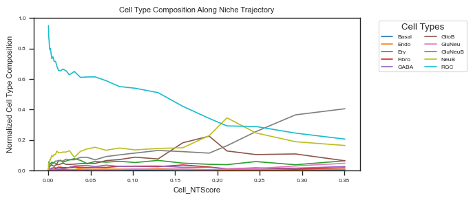
Cell type composition along the spatial trajectory reflects changes in the microenvironment.

Cell type composition change for all cells

fig, ax = plot_cell_type_composition_along_trajectory_from_anadata(
    ana_data=ana_data,  # AnaData object
    cell_types=None,  # Column name(s) in AnaData.meta_data_df that contains the cell type information.
                      # Default is None, which means all cell types in AnaData.cell_type_codes will be used.
    agg_cell_num=100,  # Number of cells to aggregate in each bin along the trajectory. Default is 10. 1 means no aggregation.
    figsize=(8,4),  # Figure size. Default is (6, 2).
    palette=None,  # Color palette for cell types. If None, use default color palette. Keys are cell types and values are colors.
    output_file_path=None  # Path to save the figure. If None, the default path
                           # {ana_data.options.output}/lineplot_raw_cell_type_composition_along_trajectory.pdf is used. 
                           # If ana_data.options.output is also None, the figure will not be saved and the function 
                           # will return the figure and axes objects instead.
)

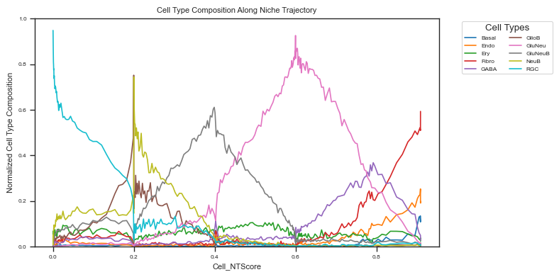
We observe that the dominant cell type shifts along the spatial trajectory, from RGCs (undifferentiated cells) to NeuB, GluNeuB, and ultimately to fully differentiated cells such as GluNeu and GABA neurons.

Cell type composition change around RGCs only

# create data_df
data_df = ana_data.meta_data_df.copy()
data_df = data_df.join(1 - ana_data.NT_score['Cell_NTScore'] if hasattr(ana_data.options, 'reverse')
                       and ana_data.options.reverse else ana_data.NT_score['Cell_NTScore'])
data_df = data_df.join(ana_data.cell_type_composition)

# filtering with cell type
data_df = data_df[data_df['Cell_Type'] == 'RGC']

cell_types = ana_data.cell_type_codes['Cell_Type'].values.tolist()

fig ,ax = plot_cell_type_composition_along_trajectory(
    data_df=data_df,
    trajectory='Cell_NTScore',
    cell_types=cell_types, # type: ignore
    agg_cell_num=100,
    figsize=(7,3),
    palette=None,
    output_file_path=None,
)

In E14.5, RGCs are primarily located within RGC-dominant microenvironments. Along the spatial trajectory, the proportion of RGCs gradually decreases, while NeuB and GluNeuB cells increase sequentially. We will explore the features associated with this dynamic in the following sections.

Differentiation potency along trajectory

We can investigate differentiation potency by using Moscot to predict the potential offspring of RGCs in the next stage (E16.5). The Moscot output have been loaded in previous section.

Selecting RGCs from Moscot results and aggregate replicates information

target_cells = ana_data.meta_data_df[(ana_data.meta_data_df['Cell_Type'] == 'RGC') & (ana_data.meta_data_df['Sample'] == 'E14_E1S3')]

def ot_res_process(ot_res):
    ot_res = ot_res.loc[ot_res.index.isin(ana_data.meta_data_df.index),
                       ot_res.columns.isin(ana_data.meta_data_df.index)]
    top_5_indices = ot_res.apply(lambda row: row.nlargest(5).index, axis=1)
    top_5_cell_types = top_5_indices.apply(lambda x: ana_data.meta_data_df.loc[x, 'Cell_Type'])
    summary_df = top_5_cell_types.apply(lambda x: x.value_counts(), axis=1).fillna(0).astype(int)
    summary_df = summary_df.loc[target_cells.index]
    summary_df = summary_df.div(summary_df.sum(axis=1).values, axis=0)
    summary_df = summary_df.join(1-ana_data.NT_score['Cell_NTScore'] if hasattr(ana_data.options, 'reverse')
                       and ana_data.options.reverse else ana_data.NT_score['Cell_NTScore'])
    
    return summary_df
    

summary_df_1 = ot_res_process(ot_res1)
summary_df_1.head()

	Basal	Endo	Ery	Fibro	GABA	GlioB	GluNeu	GluNeuB	NeuB	RGC	Cell_NTScore
Cell_ID
E14_E1S3_171289	0.0	0.0	0.0	0.2	0.4	0.0	0.0	0.0	0.0	0.4	0.105795
E14_E1S3_171863	0.0	0.0	0.0	0.0	0.0	0.0	0.0	0.8	0.0	0.2	0.020465
E14_E1S3_171967	0.0	0.0	0.0	0.0	0.0	0.4	0.0	0.6	0.0	0.0	0.019447
E14_E1S3_171983	0.0	0.0	0.0	0.0	0.2	0.0	0.0	0.8	0.0	0.0	0.041343
E14_E1S3_172013	0.0	0.0	0.0	0.0	0.2	0.0	0.0	0.4	0.0	0.4	0.023282

E14_RGC_metacell_diff_p_1_df = construct_meta_cell_along_trajectory(
    meta_data_df = summary_df_1,
    trajectory = 'Cell_NTScore',
    n_cells = 10)
E14_RGC_metacell_diff_p_1_df.head()

	Basal	Endo	Ery	Fibro	GABA	GlioB	GluNeu	GluNeuB	NeuB	RGC	Cell_NTScore
Cell_ID
E14_E1S3_173789	0.0	0.0	0.00	0.00	0.02	0.16	0.00	0.14	0.30	0.38	0.000230
E14_E1S3_173259	0.0	0.0	0.00	0.02	0.00	0.16	0.02	0.22	0.20	0.38	0.000240
E14_E1S3_174106	0.0	0.0	0.02	0.00	0.00	0.06	0.02	0.24	0.16	0.50	0.000250
E14_E1S3_173417	0.0	0.0	0.00	0.02	0.08	0.14	0.02	0.30	0.04	0.40	0.000266
E14_E1S3_173284	0.0	0.0	0.06	0.00	0.08	0.10	0.02	0.24	0.16	0.34	0.000285

summary_df_2 = ot_res_process(ot_res2)
E14_RGC_metacell_diff_p_2_df = construct_meta_cell_along_trajectory(
    meta_data_df = summary_df_2,
    trajectory = 'Cell_NTScore',
    n_cells = 10)
E14_RGC_metacell_diff_p_2_df.head()

	Basal	Endo	Ery	Fibro	GABA	GlioB	GluNeu	GluNeuB	NeuB	RGC	Cell_NTScore
Cell_ID
E14_E1S3_173789	0.0	0.0	0.02	0.06	0.12	0.12	0.02	0.06	0.10	0.50	0.000230
E14_E1S3_173259	0.0	0.0	0.00	0.00	0.08	0.14	0.00	0.04	0.14	0.60	0.000240
E14_E1S3_174106	0.0	0.0	0.02	0.04	0.04	0.00	0.02	0.08	0.12	0.68	0.000250
E14_E1S3_173417	0.0	0.0	0.02	0.00	0.04	0.14	0.00	0.08	0.06	0.66	0.000266
E14_E1S3_173284	0.0	0.0	0.00	0.02	0.10	0.12	0.02	0.08	0.08	0.58	0.000285

summary_df_3 = ot_res_process(ot_res3)
E14_RGC_metacell_diff_p_3_df = construct_meta_cell_along_trajectory(
    meta_data_df = summary_df_3,
    trajectory = 'Cell_NTScore',
    n_cells = 10)
E14_RGC_metacell_diff_p_3_df.head()

	Basal	Endo	Ery	Fibro	GABA	GlioB	GluNeu	GluNeuB	NeuB	RGC	Cell_NTScore
Cell_ID
E14_E1S3_173789	0.00	0.0	0.00	0.12	0.02	0.02	0.04	0.10	0.04	0.66	0.000230
E14_E1S3_173259	0.02	0.0	0.02	0.04	0.02	0.02	0.00	0.06	0.02	0.80	0.000240
E14_E1S3_174106	0.00	0.0	0.12	0.06	0.08	0.02	0.02	0.08	0.00	0.62	0.000250
E14_E1S3_173417	0.02	0.0	0.04	0.06	0.04	0.02	0.04	0.14	0.00	0.64	0.000266
E14_E1S3_173284	0.00	0.0	0.02	0.06	0.12	0.04	0.08	0.20	0.00	0.48	0.000285

E14_RGC_metacell_diff_p_1_melted_df = E14_RGC_metacell_diff_p_1_df.melt(
    id_vars='Cell_NTScore',
    value_vars=E14_RGC_metacell_diff_p_1_df.columns.tolist()[:-1],
    var_name='Cell type',
    value_name='Proportion')
E14_RGC_metacell_diff_p_1_melted_df['replicate'] = ['rep1'] * E14_RGC_metacell_diff_p_1_melted_df.shape[0]
E14_RGC_metacell_diff_p_1_melted_df.head()

	Cell_NTScore	Cell type	Proportion	replicate
0	0.000230	Basal	0.0	rep1
1	0.000240	Basal	0.0	rep1
2	0.000250	Basal	0.0	rep1
3	0.000266	Basal	0.0	rep1
4	0.000285	Basal	0.0	rep1

E14_RGC_metacell_diff_p_2_melted_df = E14_RGC_metacell_diff_p_2_df.melt(
    id_vars='Cell_NTScore',
    value_vars=E14_RGC_metacell_diff_p_2_df.columns.tolist()[:-1],
    var_name='Cell type',
    value_name='Proportion')
E14_RGC_metacell_diff_p_2_melted_df['replicate'] = ['rep2'] * E14_RGC_metacell_diff_p_2_melted_df.shape[0]
E14_RGC_metacell_diff_p_2_melted_df.head()

	Cell_NTScore	Cell type	Proportion	replicate
0	0.000230	Basal	0.0	rep2
1	0.000240	Basal	0.0	rep2
2	0.000250	Basal	0.0	rep2
3	0.000266	Basal	0.0	rep2
4	0.000285	Basal	0.0	rep2

E14_RGC_metacell_diff_p_3_melted_df = E14_RGC_metacell_diff_p_3_df.melt(
    id_vars='Cell_NTScore',
    value_vars=E14_RGC_metacell_diff_p_3_df.columns.tolist()[:-1],
    var_name='Cell type',
    value_name='Proportion')
E14_RGC_metacell_diff_p_3_melted_df['replicate'] = ['rep3'] * E14_RGC_metacell_diff_p_3_melted_df.shape[0]
E14_RGC_metacell_diff_p_3_melted_df.head()

	Cell_NTScore	Cell type	Proportion	replicate
0	0.000230	Basal	0.00	rep3
1	0.000240	Basal	0.02	rep3
2	0.000250	Basal	0.00	rep3
3	0.000266	Basal	0.02	rep3
4	0.000285	Basal	0.00	rep3

E14_RGC_metacell_diff_p_melted = pd.concat([E14_RGC_metacell_diff_p_1_melted_df,
                                            E14_RGC_metacell_diff_p_2_melted_df,
                                            E14_RGC_metacell_diff_p_3_melted_df])
E14_RGC_metacell_diff_p_melted.head()

	Cell_NTScore	Cell type	Proportion	replicate
0	0.000230	Basal	0.0	rep1
1	0.000240	Basal	0.0	rep1
2	0.000250	Basal	0.0	rep1
3	0.000266	Basal	0.0	rep1
4	0.000285	Basal	0.0	rep1

sns.lmplot(data = E14_RGC_metacell_diff_p_melted[E14_RGC_metacell_diff_p_melted['Cell type'].isin(['RGC', 'NeuB'])],
           x = 'Cell_NTScore',
           y = 'Proportion',
           hue = 'Cell type',
           scatter_kws={'edgecolor': None},
           ci=95,
          )

<seaborn.axisgrid.FacetGrid at 0x151b22d76110>

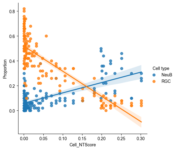
Along the spatial trajectory, the probability of RGCs maintaining their identity decreases, while the probability of their differentiation into NeuB increases.

Gene expression changes along spatial trajectory

Next, we explore gene expression dynamics along the spatial trajectory.

E14_RGC_gene_exp_df = E14_RGC_scaled_exp.join(1 - ana_data.NT_score['Cell_NTScore'] if hasattr(ana_data.options, 'reverse')
                       and ana_data.options.reverse else ana_data.NT_score['Cell_NTScore'])

# The meta-cell could reduce the noise here
E14_RGC_gene_exp_metacell_data_df = construct_meta_cell_along_trajectory(
    meta_data_df = E14_RGC_gene_exp_df,
    trajectory = 'Cell_NTScore',
    n_cells = 10
)
E14_RGC_gene_exp_metacell_data_df.head()

	0610005C13Rik	0610006L08Rik	0610009B22Rik	0610009O20Rik	0610010F05Rik	0610010K14Rik	0610012G03Rik	0610025J13Rik	0610030E20Rik	0610031O16Rik	...	Zwilch	Zwint	Zxdb	Zxdc	Zyg11a	Zyg11b	Zyx	Zzef1	Zzz3	Cell_NTScore
Cell_ID
E14_E1S3_173789	-0.036511	-0.008535	-0.198124	-0.106792	-0.239179	-0.098032	0.516922	-0.025192	-0.088172	-0.008486	...	0.938360	0.371673	-0.073764	-0.117644	-0.043855	-0.223836	-0.21233	-0.148131	0.353277	0.000230
E14_E1S3_173259	-0.036511	-0.008535	-0.198124	-0.106792	0.117162	0.537851	-0.049493	-0.025192	-0.088172	-0.008486	...	-0.068489	0.011324	-0.073764	-0.117644	-0.043855	-0.223836	-0.21233	0.946734	-0.199425	0.000240
E14_E1S3_174106	-0.036511	-0.008535	-0.198124	-0.106792	-0.239179	-0.093338	0.008216	-0.025192	-0.088172	-0.008486	...	-0.068489	-0.117173	0.933613	-0.117644	-0.043855	-0.223836	-0.21233	-0.148131	0.234650	0.000250
E14_E1S3_173417	-0.036511	-0.008535	-0.198124	-0.106792	-0.239179	-0.064664	-0.321011	-0.025192	-0.088172	-0.008486	...	-0.068489	-0.081511	-0.073764	-0.117644	-0.043855	-0.223836	-0.21233	-0.148131	-0.199425	0.000266
E14_E1S3_173284	-0.036511	-0.008535	-0.198124	-0.106792	-0.239179	0.321239	-0.321011	-0.025192	-0.088172	-0.008486	...	-0.068489	-0.389927	-0.073764	-0.117644	-0.043855	-0.223836	-0.21233	-0.148131	-0.199425	0.000285

5 rows × 23945 columns

gene_correlated_df = cal_features_correlation_along_trajectory(
    data_df = E14_RGC_gene_exp_metacell_data_df,
    trajectory = 'Cell_NTScore',
    rho_threshold=0.4,
    p_val_threshold=0.01
)
print(gene_correlated_df.shape)

/sc/arion/work/wangw32/conda-env/envs/ONTraC/lib/python3.11/site-packages/ONTraC/analysis/trajectory.py:102: ConstantInputWarning: An input array is constant; the correlation coefficient is not defined.
  rho, p_val = pearsonr(data_df[trajectory], data_df[feat])

(109, 2)

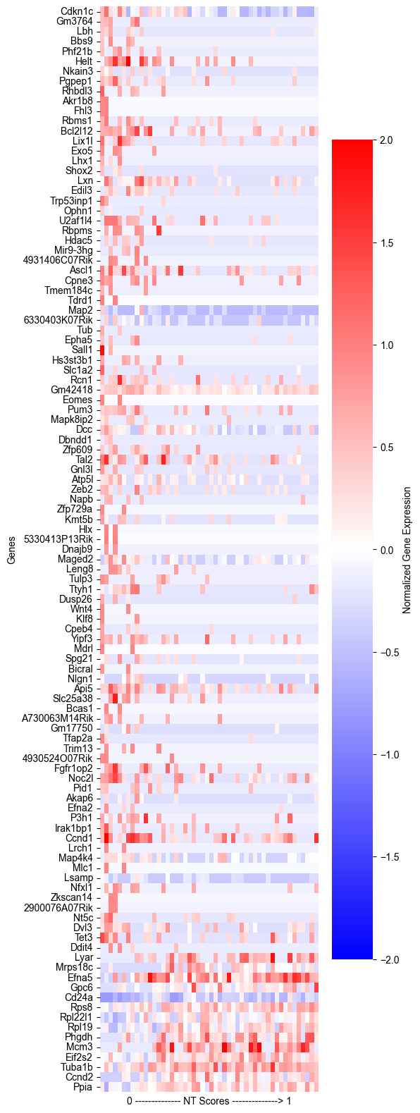
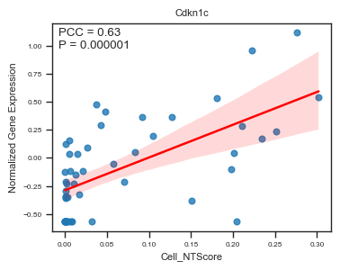
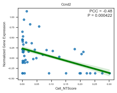
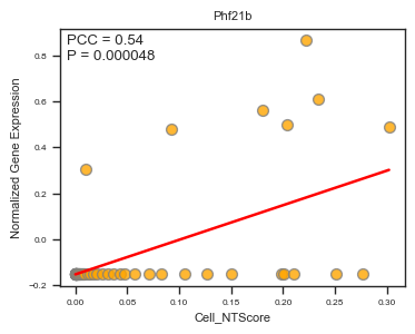
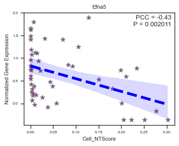
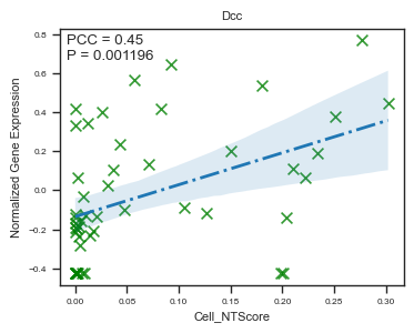
We identified 109 genes whose expression levels are significantly correlated with cell-level NT scores. Here, we highlight six representative genes that are strongly associated with neuronal differentiation and maturation.

gene_correlated_df.head()

	PCC	P_Value
Feature
Cdkn1c	0.629617	9.666948e-07
Gm3764	0.623302	1.333598e-06
Lbh	0.618297	1.712368e-06
Bbs9	0.550067	3.502920e-05
Phf21b	0.542046	4.788367e-05

Different Filtering Parameters

You can also select top N genes by following command:

cal_features_correlation_along_trajectory(
    data_df = E14_RGC_gene_exp_metacell_data_df,
    trajectory = 'Cell_NTScore',
    top_n=5,
    rho_threshold=0.4,
    p_val_threshold=0.01
)

/sc/arion/work/wangw32/conda-env/envs/ONTraC/lib/python3.11/site-packages/ONTraC/analysis/trajectory.py:102: ConstantInputWarning: An input array is constant; the correlation coefficient is not defined.
  rho, p_val = pearsonr(data_df[trajectory], data_df[feat])

	PCC	P_Value
Feature
Cdkn1c	0.629617	9.666948e-07
Gm3764	0.623302	1.333598e-06
Lbh	0.618297	1.712368e-06
Bbs9	0.550067	3.502920e-05
Phf21b	0.542046	4.788367e-05
Mcm3	-0.453214	9.492690e-04
Eif2s2	-0.456194	8.696506e-04
Tuba1b	-0.470727	5.608145e-04
Ccnd2	-0.479827	4.218648e-04
Ppia	-0.484622	3.619282e-04

Heatmap Showing Trajectory-Associated Genes

filtered_metacell_gene_exp_df = E14_RGC_gene_exp_metacell_data_df.loc[:,gene_correlated_df.index]
filtered_metacell_gene_exp_df.head()

Feature	Cdkn1c	Gm3764	Lbh	Bbs9	Phf21b	Helt	Nkain3	Pgpep1	Rhbdl3	Akr1b8	...	Cd24a	Rps8	Rpl22l1	Rpl19	Phgdh	Mcm3	Eif2s2	Tuba1b	Ccnd2	Ppia
Cell_ID
E14_E1S3_173789	-0.126359	-0.152949	0.148899	-0.111262	-0.150273	-0.108984	-0.237243	-0.167096	-0.122761	-0.052675	...	-0.418015	0.575271	0.220949	0.309830	0.164429	-0.159499	0.234015	0.449034	0.433422	0.543230
E14_E1S3_173259	-0.570163	-0.152949	-0.192196	-0.111262	-0.150273	-0.108984	-0.237243	-0.167096	-0.122761	-0.052675	...	-0.251175	0.916426	0.492244	0.625080	1.361812	0.350744	0.431511	0.532895	0.642079	0.112190
E14_E1S3_174106	-0.570163	-0.152949	-0.192196	-0.111262	-0.150273	-0.108984	-0.237243	-0.167096	-0.122761	-0.052675	...	-0.207797	0.531247	-0.033359	0.499405	1.262983	1.341346	0.214287	0.608114	-0.371306	0.839393
E14_E1S3_173417	-0.570163	-0.152949	-0.192196	-0.111262	-0.150273	-0.108984	-0.237243	-0.167096	-0.122761	-0.052675	...	-0.593854	0.697930	0.274315	-0.226063	-0.240031	1.718599	-0.099978	0.528772	0.449835	0.103245
E14_E1S3_173284	-0.570163	-0.152949	-0.192196	-0.111262	-0.150273	-0.108984	-0.237243	-0.167096	-0.122761	-0.052675	...	-0.371482	0.731672	0.595815	0.640199	0.716297	1.006487	0.340025	0.822160	0.210475	0.089651

5 rows × 109 columns

fig, ax = plt.subplots(figsize=(5, 20))
sns.heatmap(filtered_metacell_gene_exp_df.iloc[::-1,].T,
            cmap='bwr',
            vmin=-2,
            vmax=2,
            cbar_kws={'label': 'Normalized Gene Expression'},
            ax=ax)
ax.set_xticks([])
ax.set_xlabel('0 -------------- NT Scores --------------> 1')
ax.set_ylabel('Genes')

Text(33.222222222222214, 0.5, 'Genes')

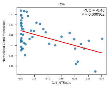
Diagnosis of Selected Genes

fig, ax = plot_scatter_feat_along_trajectory(
    data_df = E14_RGC_gene_exp_metacell_data_df,
    trajectory = 'Cell_NTScore',
    feature = 'Ppia',
    fit_reg = True,
    annotate_pos = 'upper right',
    figszie = (4,3),
    ylabel = 'Normalized Gene Expression',
)

fig, ax = plot_scatter_feat_along_trajectory(
    data_df = E14_RGC_gene_exp_metacell_data_df,
    trajectory = 'Cell_NTScore',
    feature = 'Cdkn1c',
    fit_reg = True,
    annotate_pos = 'upper left',
    figszie = (4,3),
    ylabel = 'Normalized Gene Expression',
    ci=95,  # Size of the confidence interval for the regression estimate
)

fig, ax = plot_scatter_feat_along_trajectory(
    data_df = E14_RGC_gene_exp_metacell_data_df,
    trajectory = 'Cell_NTScore',
    feature = 'Ccnd2',
    fit_reg = True,
    annotate_pos = 'upper right',
    figszie = (4,3),
    ylabel = 'Normalized Gene Expression',
    line_kws = {'color': 'green', 'lw': 4},  # line parameters
    ci=70,  # Size of the confidence interval for the regression estimate
)

fig, ax = plot_scatter_feat_along_trajectory(
    data_df = E14_RGC_gene_exp_metacell_data_df,
    trajectory = 'Cell_NTScore',
    feature = 'Phf21b',
    fit_reg = True,
    annotate_pos = 'upper left',
    figszie = (4,3),
    ylabel = 'Normalized Gene Expression',
    scatter_kws = {'color': 'orange', 'edgecolor': 'gray', 's': 50},  # scatter parameters
)

fig, ax = plot_scatter_feat_along_trajectory(
    data_df = E14_RGC_gene_exp_metacell_data_df,
    trajectory = 'Cell_NTScore',
    feature = 'Efna5',
    fit_reg = True,
    annotate_pos = 'upper right',
    figszie = (4,3),
    ylabel = 'Normalized Gene Expression',
    scatter_kws = {'color': 'purple', 'edgecolor': 'gray', 's': 50},  # scatter parameters
    line_kws = {'color': 'blue', 'lw': 4, 'ls': '--'},  # line parameters
    ci = 95,  # Size of the confidence interval for the regression estimate
    marker = '*',  # Marker to use for the scatterplot glyphs.
)

fig, ax = plot_scatter_feat_along_trajectory(
    data_df = E14_RGC_gene_exp_metacell_data_df,
    trajectory = 'Cell_NTScore',
    feature = 'Dcc',
    fit_reg = True,
    annotate_pos = 'upper left',
    figszie = (4,3),
    ylabel = 'Normalized Gene Expression',
    scatter_kws = {'color': 'green', 's': 50},  # scatter parameters
    line_kws = {'color': 'C0', 'lw': 2, 'ls': '-.'},  # line parameters
    ci = 95,  # Size of the confidence interval for the regression estimate.
    marker = 'x',  # Marker to use for the scatterplot glyphs.
)

Gene Set Enrichment Analysis (GSEA)

# keep all genes while calculate correlation
all_gene_correlation_df = cal_features_correlation_along_trajectory(
    data_df = E14_RGC_gene_exp_metacell_data_df,
    trajectory = 'Cell_NTScore',
)
print(all_gene_correlation_df.shape)

/sc/arion/work/wangw32/conda-env/envs/ONTraC/lib/python3.11/site-packages/ONTraC/analysis/trajectory.py:102: ConstantInputWarning: An input array is constant; the correlation coefficient is not defined.
  rho, p_val = pearsonr(data_df[trajectory], data_df[feat])

(13636, 2)

all_gene_correlation_df.head()

	PCC	P_Value
Feature
Cdkn1c	0.629617	9.666948e-07
Gm3764	0.623302	1.333598e-06
Lbh	0.618297	1.712368e-06
Bbs9	0.550067	3.502920e-05
Phf21b	0.542046	4.788367e-05

all_gene_correlation_df.tail()

	PCC	P_Value
Feature
Mcm3	-0.453214	0.000949
Eif2s2	-0.456194	0.000870
Tuba1b	-0.470727	0.000561
Ccnd2	-0.479827	0.000422
Ppia	-0.484622	0.000362

reject, qvals, _, _ = multipletests(all_gene_correlation_df['P_Value'].values, alpha=0.05, method="fdr_bh")
all_gene_correlation_df.loc[:,'FDR Q-Value'] = qvals
all_gene_correlation_df.head()

	PCC	P_Value	FDR Q-Value
Feature
Cdkn1c	0.629617	9.666948e-07	0.007783
Gm3764	0.623302	1.333598e-06	0.007783
Lbh	0.618297	1.712368e-06	0.007783
Bbs9	0.550067	3.502920e-05	0.119415
Phf21b	0.542046	4.788367e-05	0.130588

all_gene_correlation_df.tail()

	PCC	P_Value	FDR Q-Value
Feature
Mcm3	-0.453214	0.000949	0.311213
Eif2s2	-0.456194	0.000870	0.311213
Tuba1b	-0.470727	0.000561	0.275297
Ccnd2	-0.479827	0.000422	0.225432
Ppia	-0.484622	0.000362	0.224330

# corrected, only one columns should list here, otherwise, there are multiple ranks as inputs
corr_rnk = all_gene_correlation_df.iloc[:,:1]
corr_rnk.head()

	PCC
Feature
Cdkn1c	0.629617
Gm3764	0.623302
Lbh	0.618297
Bbs9	0.550067
Phf21b	0.542046

corr_rnk.tail()

	PCC
Feature
Mcm3	-0.453214
Eif2s2	-0.456194
Tuba1b	-0.470727
Ccnd2	-0.479827
Ppia	-0.484622

pre_res = gp.prerank(rnk=corr_rnk, # or rnk = rnk,
                     gene_sets='./c5.go.bp.v7.5.1.symbols.gmt',
                     threads=4,
                     min_size=5,
                     max_size=1000,
                     permutation_num=1000, # reduce number to speed up testing
                     outdir=None, # don't write to disk
                     seed=6,
                     verbose=True, # see what's going on behind the scenes
                    )

2025-08-24 12:13:10,204 [WARNING] Duplicated values found in preranked stats: 16.66% of genes
The order of those genes will be arbitrary, which may produce unexpected results.
2025-08-24 12:13:10,204 [INFO] Parsing data files for GSEA.............................
2025-08-24 12:13:10,381 [INFO] 1188 gene_sets have been filtered out when max_size=1000 and min_size=5
2025-08-24 12:13:10,382 [INFO] 6470 gene_sets used for further statistical testing.....
2025-08-24 12:13:10,382 [INFO] Start to run GSEA...Might take a while..................
2025-08-24 12:13:10,383 [INFO] Genes are converted to uppercase.
2025-08-24 12:14:15,539 [INFO] Congratulations. GSEApy runs successfully................

res = pre_res.res2d
filter_res = res[[True if x.startswith('GOBP') else False for x in res['Term']]]
filter_res = filter_res[filter_res['NOM p-val'] < 0.05]

filter_res.head()

	Name	Term	ES	NES	NOM p-val	FDR q-val	FWER p-val	Tag %	Gene %	Lead_genes
0	prerank	GOBP_CYTOPLASMIC_TRANSLATION	-0.449215	-2.385238	0.0	0.004127	0.004	58/135	20.85%	Eif2s2;Rpl19;Rpl22l1;Rps8;Rpl3;Rps23;Rpl8;Rpl4...
1	prerank	GOBP_TRICARBOXYLIC_ACID_CYCLE	-0.624419	-2.374058	0.0	0.002579	0.004	9/27	6.50%	Idh2;Sdhd;Suclg2;Dlat;Idh3a;Mrps36;Dlst;Pdhb;Cs
2	prerank	GOBP_DNA_REPLICATION_INITIATION	-0.57303	-2.36083	0.0	0.00172	0.004	12/35	11.85%	Mcm3;Mcm5;Topbp1;Pola1;Prim2;Mcm2;Ccne2;Mcm6;M...
3	prerank	GOBP_DNA_UNWINDING_INVOLVED_IN_DNA_REPLICATION	-0.667623	-2.270939	0.0	0.006965	0.026	12/20	17.51%	Mcm3;Mcm5;Gins2;Blm;Mcm2;Mcm6;Twnk;Cdc45;Gins4...
4	prerank	GOBP_DNA_DEPENDENT_DNA_REPLICATION	-0.4078	-2.236996	0.0	0.00908	0.039	57/144	21.58%	Mcm3;Mcm5;Topbp1;Pola1;Gins2;Blm;Eme1;Rfc1;Cdk...

filter_res.sort_values('NES').head(20)

	Name	Term	ES	NES	NOM p-val	FDR q-val	FWER p-val	Tag %	Gene %	Lead_genes
0	prerank	GOBP_CYTOPLASMIC_TRANSLATION	-0.449215	-2.385238	0.0	0.004127	0.004	58/135	20.85%	Eif2s2;Rpl19;Rpl22l1;Rps8;Rpl3;Rps23;Rpl8;Rpl4...
1	prerank	GOBP_TRICARBOXYLIC_ACID_CYCLE	-0.624419	-2.374058	0.0	0.002579	0.004	9/27	6.50%	Idh2;Sdhd;Suclg2;Dlat;Idh3a;Mrps36;Dlst;Pdhb;Cs
2	prerank	GOBP_DNA_REPLICATION_INITIATION	-0.57303	-2.36083	0.0	0.00172	0.004	12/35	11.85%	Mcm3;Mcm5;Topbp1;Pola1;Prim2;Mcm2;Ccne2;Mcm6;M...
3	prerank	GOBP_DNA_UNWINDING_INVOLVED_IN_DNA_REPLICATION	-0.667623	-2.270939	0.0	0.006965	0.026	12/20	17.51%	Mcm3;Mcm5;Gins2;Blm;Mcm2;Mcm6;Twnk;Cdc45;Gins4...
4	prerank	GOBP_DNA_DEPENDENT_DNA_REPLICATION	-0.4078	-2.236996	0.0	0.00908	0.039	57/144	21.58%	Mcm3;Mcm5;Topbp1;Pola1;Gins2;Blm;Eme1;Rfc1;Cdk...
5	prerank	GOBP_DOUBLE_STRAND_BREAK_REPAIR_VIA_BREAK_INDU...	-0.78386	-2.145294	0.0	0.036972	0.174	10/11	20.09%	Mcm3;Mcm5;Gins2;Mcm2;Mcm6;Cdc45;Gins4;Mcm7;Cdc...
6	prerank	GOBP_NEGATIVE_REGULATION_OF_RNA_SPLICING	-0.572831	-2.084832	0.0	0.069129	0.338	10/25	13.52%	Srsf4;Ptbp1;Hnrnpa2b1;Srsf7;C1qbp;Sap18;Rps26;...
7	prerank	GOBP_DNA_REPLICATION	-0.351203	-2.077697	0.0	0.066808	0.37	99/253	23.39%	Mcm3;Mcm5;Set;Topbp1;Pola1;Nasp;Gins2;Blm;Rrm2...
8	prerank	GOBP_CHROMATIN_REMODELING_AT_CENTROMERE	-0.762886	-2.074276	0.0	0.062136	0.383	5/9	6.65%	Hells;Nasp;Hjurp;Mis18a;Oip5
9	prerank	GOBP_DNA_GEOMETRIC_CHANGE	-0.407036	-2.048352	0.0	0.07728	0.47	30/85	15.53%	Mcm3;Mcm5;Gins2;Blm;Dscc1;Hnrnpa2b1;Brip1;Mcm2...
10	prerank	GOBP_HISTONE_EXCHANGE	-0.635976	-2.041671	0.0	0.077008	0.495	5/16	6.65%	Nasp;Hjurp;Spty2d1;Mis18a;Oip5
11	prerank	GOBP_ATRIAL_CARDIAC_MUSCLE_CELL_TO_AV_NODE_CEL...	-0.680813	-2.04045	0.0	0.072053	0.503	9/13	20.41%	Cacna1c;Cacnb2;Trpm4;Gjc1;Gja1;Scn3b;Kcna5;Kcn...
12	prerank	GOBP_SNORNA_LOCALIZATION	-0.889979	-2.026537	0.0	0.077225	0.564	5/6	9.18%	Fbl;Nop58;Pih1d1;Prpf31;Znhit3
13	prerank	GOBP_DERMATAN_SULFATE_PROTEOGLYCAN_METABOLIC_P...	-0.838072	-2.022415	0.0	0.07532	0.582	6/7	15.40%	B3gat3;Idua;Chst12;Dsel;Csgalnact2;Chst14
15	prerank	GOBP_CENP_A_CONTAINING_CHROMATIN_ORGANIZATION	-0.82405	-1.995891	0.0	0.095268	0.679	4/7	6.65%	Nasp;Hjurp;Mis18a;Oip5
16	prerank	GOBP_POSITIVE_REGULATION_OF_PATTERN_RECOGNITIO...	-0.522305	-1.99507	0.0	0.090152	0.681	17/26	27.00%	Usp15;Rtn4;Ankrd17;Ninj1;Tirap;Hmgb1;Cav1;Ifi3...
17	prerank	GOBP_AEROBIC_RESPIRATION	-0.364381	-1.9943	0.0	0.08582	0.686	50/147	22.85%	Ndufs1;Cox5b;Ndufc2;Ide;Uqcr10;Idh2;Sdhd;Ccnb1...
18	prerank	GOBP_REGULATION_OF_DNA_DIRECTED_DNA_POLYMERASE...	-0.638066	-1.990986	0.0	0.083803	0.695	7/13	14.97%	Gins2;Dscc1;Rfc5;Gins4;Rfc3;Pcna;Polg2
19	prerank	GOBP_NEGATIVE_REGULATION_OF_MRNA_SPLICING_VIA_...	-0.582963	-1.97912	0.004662	0.092806	0.749	9/20	13.52%	Srsf4;Ptbp1;Hnrnpa2b1;Srsf7;C1qbp;Sap18;Sfswap...
20	prerank	GOBP_DOUBLE_STRAND_BREAK_REPAIR	-0.332017	-1.964585	0.0	0.105603	0.802	93/231	24.37%	Mcm3;Mcm5;Pola1;Smchd1;Nabp2;Gins2;Blm;Babam1;...

filter_res.sort_values('NES').tail(20)

	Name	Term	ES	NES	NOM p-val	FDR q-val	FWER p-val	Tag %	Gene %	Lead_genes
92	prerank	GOBP_POSITIVE_REGULATION_OF_HAIR_FOLLICLE_DEVE...	0.725166	1.743163	0.005639	1.0	1.0	3/8	4.61%	Tgfb2;Gal;Krt17
86	prerank	GOBP_REGULATION_OF_PROTEIN_LOCALIZATION_TO_CEN...	0.6737	1.750461	0.010949	1.0	1.0	6/10	11.80%	Bicd1;Cep250;Mark4;Nup62;Pard6a;Ubxn2b
83	prerank	GOBP_PLANAR_CELL_POLARITY_PATHWAY_INVOLVED_IN_...	0.661712	1.751047	0.015652	1.0	1.0	6/11	16.61%	Dvl3;Sfrp2;Fzd1;Dvl1;Nphp3;Sfrp1
77	prerank	GOBP_OLFACTORY_LOBE_DEVELOPMENT	0.498639	1.761532	0.006319	1.0	1.0	10/30	12.64%	Sall1;Eomes;Efna2;Slit1;Chd7;Srf;Erbb4;Robo1;R...
74	prerank	GOBP_REGULATION_OF_FATTY_ACID_BETA_OXIDATION	0.570444	1.76705	0.008606	1.0	1.0	8/17	15.92%	Etfbkmt;Cnr1;Abcd2;Lonp2;Irs1;Mlycd;Tysnd1;Acacb
71	prerank	GOBP_NEGATIVE_REGULATION_OF_COLLATERAL_SPROUTING	0.731298	1.773559	0.007707	1.0	1.0	6/8	16.75%	Dcc;Ptprs;Spp1;Ulk1;Epha7;Ulk2
68	prerank	GOBP_ANTERIOR_POSTERIOR_AXON_GUIDANCE	0.756514	1.780581	0.0	1.0	1.0	3/7	1.69%	Lhx1;Dcc;Lhx9
65	prerank	GOBP_REGULATION_OF_NEURON_PROJECTION_ARBORIZATION	0.621632	1.78363	0.003656	1.0	1.0	6/13	18.11%	Dvl3;Dlg4;Macf1;Dvl1;Map3k13;Ntng1
62	prerank	GOBP_NON_CANONICAL_WNT_SIGNALING_PATHWAY_VIA_M...	0.807137	1.796288	0.001919	1.0	1.0	3/6	0.70%	Wnt4;Dvl3;Nkd1
58	prerank	GOBP_FEEDING_BEHAVIOR	0.448003	1.800532	0.002899	1.0	1.0	15/53	12.48%	Helt;Dach1;Cck;Cnr1;Lepr;Ttc21b;Npy;Gal;Fyn;Po...
57	prerank	GOBP_SPINAL_CORD_ASSOCIATION_NEURON_DIFFERENTI...	0.802871	1.804829	0.003683	1.0	1.0	4/6	10.59%	Lhx1;Ascl1;Gsx1;Tal1
51	prerank	GOBP_METANEPHRIC_NEPHRON_DEVELOPMENT	0.544978	1.826752	0.001715	1.0	0.999	10/26	18.22%	Lhx1;Sall1;Wnt4;Tcf21;Pkd2;Tfap2b;Agtr2;Sox9;L...
45	prerank	GOBP_CALCIUM_DEPENDENT_CELL_CELL_ADHESION_VIA_...	0.545783	1.843529	0.001623	1.0	0.999	12/23	19.58%	Nlgn1;Arvcf;Cdh2;Cdh8;Dchs1;Atp2c1;Cdh9;Cdh13;...
44	prerank	GOBP_DORSAL_SPINAL_CORD_DEVELOPMENT	0.713258	1.851775	0.001795	1.0	0.998	5/10	16.04%	Lhx1;Ascl1;Gsx1;Tal1;Prox1
43	prerank	GOBP_POSITIVE_REGULATION_OF_PROTEIN_LOCALIZATI...	0.793517	1.855019	0.005455	1.0	0.998	5/7	9.18%	Bicd1;Cep250;Mark4;Nup62;Pard6a
40	prerank	GOBP_GLYCOSIDE_METABOLIC_PROCESS	0.681614	1.858309	0.003676	1.0	0.996	6/12	16.68%	Gla;Gba2;Fuca2;Cbr4;Abhd10;Fuca1
38	prerank	GOBP_DIGESTIVE_SYSTEM_DEVELOPMENT	0.429413	1.87548	0.0	1.0	0.983	35/94	21.07%	Cdkn1c;Shox2;Ascl1;Sall1;Hlx;Tcf21;Hip1r;Gata4...
36	prerank	GOBP_AUTOPHAGY_OF_NUCLEUS	0.63459	1.879821	0.001695	1.0	0.98	8/15	18.20%	Atg9a;Atg7;Atg2a;Ulk1;Rb1cc1;Ulk2;Wipi2;Wdr45
27	prerank	GOBP_GLYCOSIDE_CATABOLIC_PROCESS	0.778249	1.928485	0.0	1.0	0.887	5/8	16.68%	Gla;Gba2;Fuca2;Abhd10;Fuca1
14	prerank	GOBP_GOLGI_TO_LYSOSOME_TRANSPORT	0.763518	2.009531	0.0	0.926462	0.553	4/10	7.08%	Ehd3;Ccdc91;Sort1;Rbsn

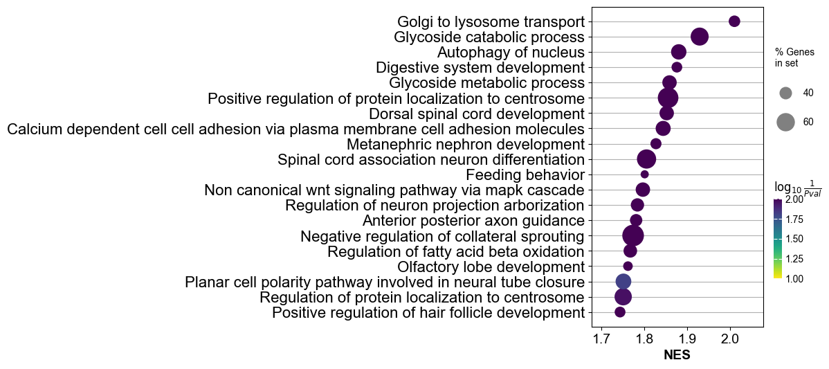
plot_data = filter_res.sort_values('NES').tail(20)
plot_data['Term'] = [x.split('_',1)[1].replace('_', ' ').capitalize() for x in plot_data['Term']]

gp.dotplot(plot_data,column="NOM p-val",top_term=20)

/sc/arion/work/wangw32/conda-env/envs/ONTraC/lib/python3.11/site-packages/gseapy/plot.py:738: FutureWarning: Downcasting behavior in `replace` is deprecated and will be removed in a future version. To retain the old behavior, explicitly call `result.infer_objects(copy=False)`. To opt-in to the future behavior, set `pd.set_option('future.no_silent_downcasting', True)`
  df[self.colname] = df[self.colname].replace(0, np.nan).bfill()

<Axes: xlabel='NES'>

plot_data = filter_res.sort_values('NES').head(20)
plot_data['Term'] = [x.split('_',1)[1].replace('_', ' ').capitalize() for x in plot_data['Term']]

gp.dotplot(plot_data,column="NOM p-val",top_term=20)

/sc/arion/work/wangw32/conda-env/envs/ONTraC/lib/python3.11/site-packages/gseapy/plot.py:738: FutureWarning: Downcasting behavior in `replace` is deprecated and will be removed in a future version. To retain the old behavior, explicitly call `result.infer_objects(copy=False)`. To opt-in to the future behavior, set `pd.set_option('future.no_silent_downcasting', True)`
  df[self.colname] = df[self.colname].replace(0, np.nan).bfill()

<Axes: xlabel='NES'>

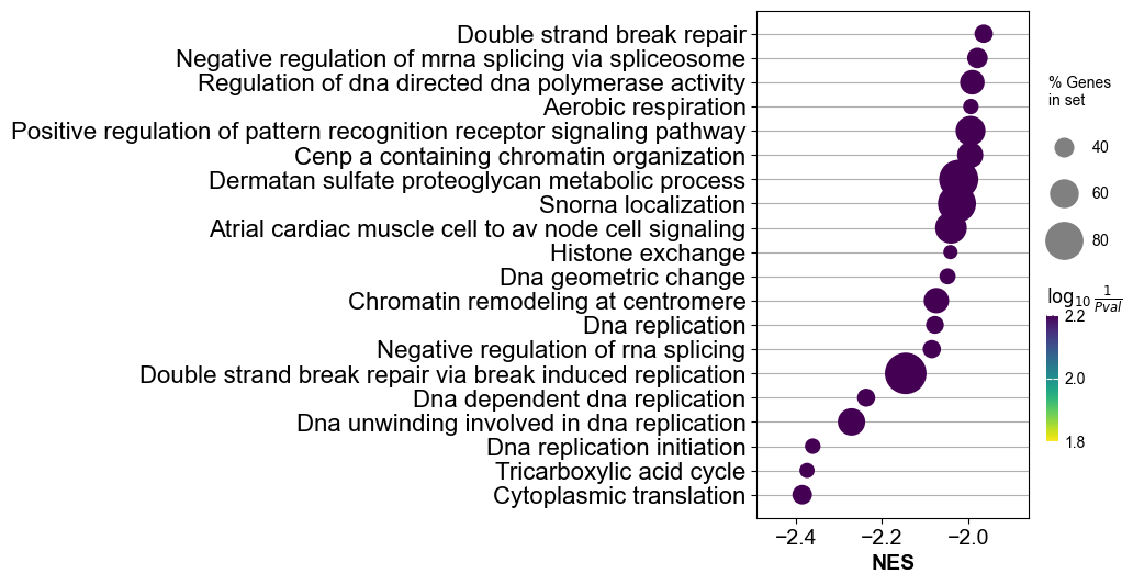
A negative NES indicates that genes associated with a given Gene Ontology (GO) term are highly expressed at the start of the trajectory (i.e., cells with low NT scores). For example, enrichment of DNA replication–related terms aligns with the potential of these cells to be preserved as RGCs in the next developmental stage (E16.5).

A positive NES indicates that GO term–associated genes are highly expressed at the end of the trajectory (i.e., cells with high NT scores). Enrichment of terms related to neuron differentiation and CNS development corresponds to the potential differentiation of RGCs into mature neuronal states by E16.5.

Regulon activity changes along spatial trajectory

To gain mechanistic insights, we performed gene regulatory network (GRN) analysis using the SCENIC workflow and explore regulon activity changes along spatial trajectory.

E14_RGC_regulon_aucell_df = regulon_aucell_df.loc[target_cells.index]
E14_RGC_regulon_aucell_df = E14_RGC_regulon_aucell_df.join(1-ana_data.NT_score['Cell_NTScore'] if hasattr(ana_data.options, 'reverse')
                       and ana_data.options.reverse else ana_data.NT_score['Cell_NTScore'])
E14_RGC_regulon_aucell_df.head()

	Ahr	Alx1	Alx3	Alx4	Ar	Arid3a	Arntl2	Arx	Atf1	Atf3	...	Zfp874b	Zfp941	Zfp944	Zfp979	Zic1	Zkscan14	Zkscan16	Zscan20	Zxdc	Cell_NTScore
Cell_ID
E14_E1S3_171289	0.0	0.015500	0.014530	0.000000	0.0	0.003071	0.000000	0.072864	0.0	0.156601	...	0.001970	0.000000	0.0	0.0	0.026855	0.056960	0.023259	0.0	0.0	0.105795
E14_E1S3_171863	0.0	0.018301	0.017757	0.032068	0.0	0.003840	0.000000	0.000000	0.0	0.169815	...	0.004407	0.000000	0.0	0.0	0.092449	0.063594	0.026734	0.0	0.0	0.020465
E14_E1S3_171967	0.0	0.011018	0.009434	0.000000	0.0	0.001884	0.000000	0.071136	0.0	0.137201	...	0.018034	0.085787	0.0	0.0	0.033001	0.046866	0.017807	0.0	0.0	0.019447
E14_E1S3_171983	0.0	0.020709	0.000000	0.003596	0.0	0.000000	0.020299	0.099791	0.0	0.034300	...	0.000000	0.000000	0.0	0.0	0.054828	0.000000	0.000000	0.0	0.0	0.041343
E14_E1S3_172013	0.0	0.009773	0.008186	0.000000	0.0	0.001552	0.228530	0.000000	0.0	0.131016	...	0.000000	0.000000	0.0	0.0	0.045381	0.043549	0.016186	0.0	0.0	0.023282

5 rows × 305 columns

E14_RGC_regulon_aucell_metacell_data_df = construct_meta_cell_along_trajectory(meta_data_df = E14_RGC_regulon_aucell_df,
                                                                trajectory = 'Cell_NTScore',
                                                                n_cells = 10)
E14_RGC_regulon_aucell_metacell_data_df.head()

	Ahr	Alx1	Alx3	Alx4	Ar	Arid3a	Arntl2	Arx	Atf1	Atf3	...	Zfp874b	Zfp941	Zfp944	Zfp979	Zic1	Zkscan14	Zkscan16	Zscan20	Zxdc	Cell_NTScore
Cell_ID
E14_E1S3_173789	0.0	0.012552	0.019366	0.011585	0.000000	0.014612	0.004832	0.026460	0.0	0.138414	...	0.019770	0.0	0.0	0.000000	0.079209	0.051178	0.022155	0.0	0.0	0.000230
E14_E1S3_173259	0.0	0.019238	0.021671	0.014015	0.000000	0.003680	0.004246	0.011797	0.0	0.111139	...	0.017413	0.0	0.0	0.000000	0.055038	0.033917	0.016856	0.0	0.0	0.000240
E14_E1S3_174106	0.0	0.010374	0.022217	0.004985	0.014738	0.008334	0.023277	0.013118	0.0	0.117493	...	0.002832	0.0	0.0	0.015804	0.068224	0.063113	0.023028	0.0	0.0	0.000250
E14_E1S3_173417	0.0	0.024025	0.014273	0.005424	0.000000	0.005799	0.005877	0.000000	0.0	0.157988	...	0.002603	0.0	0.0	0.000000	0.046749	0.056830	0.028127	0.0	0.0	0.000266
E14_E1S3_173284	0.0	0.016657	0.011069	0.011577	0.014097	0.004353	0.021781	0.049954	0.0	0.122188	...	0.008053	0.0	0.0	0.019991	0.072346	0.039267	0.028010	0.0	0.0	0.000285

5 rows × 305 columns

regulon_correlated_df = cal_features_correlation_along_trajectory(
    data_df = E14_RGC_regulon_aucell_metacell_data_df,
    trajectory = 'Cell_NTScore',
    rho_threshold=0.4,
    p_val_threshold=0.01
)
print(regulon_correlated_df.shape)

(10, 2)

/sc/arion/work/wangw32/conda-env/envs/ONTraC/lib/python3.11/site-packages/ONTraC/analysis/trajectory.py:102: ConstantInputWarning: An input array is constant; the correlation coefficient is not defined.
  rho, p_val = pearsonr(data_df[trajectory], data_df[feat])

regulon_correlated_df.head()

	PCC	P_Value
Feature
Nfatc4	0.525306	0.000090
Lhx2	0.501632	0.000206
Neurod1	0.476846	0.000464
Sox6	0.414478	0.002767
Tcf7l2	0.402664	0.003743

Diagnosis of Selected Regulons

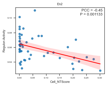
fig, ax = plot_scatter_feat_along_trajectory(
    data_df = E14_RGC_regulon_aucell_metacell_data_df,
    trajectory = 'Cell_NTScore',
    feature = 'En2',
    fit_reg = True,
    annotate_pos = 'upper right',
    figszie = (4,3),
    ylabel = 'Regulon Activity',
    ci = 95,
)

fig, ax = plot_scatter_feat_along_trajectory(
    data_df = E14_RGC_regulon_aucell_metacell_data_df,
    trajectory = 'Cell_NTScore',
    feature = 'Hes6',
    fit_reg = True,
    annotate_pos = 'upper right',
    figszie = (4,3),
    ylabel = 'Regulon Activity',
    ci = 95,
)

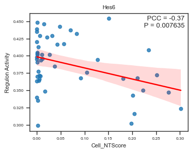
We identified several regulons whose activity scores are significantly correlated with cell-level NT scores (spatial trajectory).

Session Info

import session_info

session_info.show()

Click to view session information

-----
ONTraC              1.2.2
gseapy              1.1.5
matplotlib          3.8.4
numpy               1.26.4
pandas              2.2.1
requests            2.31.0
scipy               1.14.1
seaborn             0.13.2
session_info        1.0.0
statsmodels         0.14.4
-----

Click to view modules imported as dependencies

PIL                 10.3.0
asttokens           NA
certifi             2024.02.02
charset_normalizer  3.3.2
colorama            0.4.6
comm                0.2.2
cycler              0.12.1
cython_runtime      NA
dateutil            2.9.0.post0
debugpy             1.8.1
decorator           5.1.1
executing           2.0.1
idna                3.7
ipykernel           6.29.4
jedi                0.19.1
kiwisolver          1.4.5
matplotlib_inline   0.1.7
mpl_toolkits        NA
networkx            3.3
packaging           24.0
parso               0.8.4
patsy               0.5.6
platformdirs        4.2.1
prompt_toolkit      3.0.43
psutil              5.9.8
pure_eval           0.2.2
pydev_ipython       NA
pydevconsole        NA
pydevd              2.9.5
pydevd_file_utils   NA
pydevd_plugins      NA
pydevd_tracing      NA
pygments            2.17.2
pyparsing           3.1.2
pytz                2024.1
six                 1.16.0
stack_data          0.6.3
tornado             6.4
traitlets           5.14.3
typing_extensions   NA
urllib3             2.2.1
wcwidth             0.2.13
yaml                6.0.1
zmq                 26.0.2

-----
IPython             8.23.0
jupyter_client      8.6.1
jupyter_core        5.7.2
-----
Python 3.11.9 | packaged by conda-forge | (main, Apr 19 2024, 18:36:13) [GCC 12.3.0]
Linux-5.14.0-427.13.1.el9_4.x86_64-x86_64-with-glibc2.34
-----
Session information updated at 2025-08-24 12:14