Multi-sample conparison

Notes

This notebook demonstrates ONTraC’s ability to create consistent spatial trajectories across multiple samples/slices.

• We assume that you have installed ONTraC according to the Installation Tutorial and open this notebook using installed Python kernel (Python 3.11 (ONTraC)).

• The ONTraC running process could be found at our example tutorial

Load Modules

import os
import sys
import requests
import zipfile

import numpy as np
import pandas as pd

from scipy.stats import spearmanr

import matplotlib as mpl
import matplotlib.gridspec as gridspec
from matplotlib.lines import Line2D

mpl.rcParams['pdf.fonttype'] = 42
mpl.rcParams['ps.fonttype'] = 42
mpl.rcParams['font.family'] = 'Arial'
import matplotlib.pyplot as plt
import seaborn as sns

from ONTraC.analysis.data import AnaData

import session_info

Download Pre-processed Data

import requests

# URL of the file
url = "https://zenodo.org/records/15571644/files/MERFISH_data.zip"

# Local file path to save the file
file_path = "./MERFISH_data.zip"

try:
    # Send a GET request to the URL
    response = requests.get(url)
    response.raise_for_status()  # Check if the request was successful

    # Write the content to the file
    with open(file_path, "wb") as file:
        file.write(response.content)

    print(f"File downloaded and saved to {file_path}")
except requests.exceptions.RequestException as e:
    print(f"An error occurred: {e}")

File downloaded and saved to ./MERFISH_data.zip

import zipfile

# Path to the zip file
zip_file_path = "MERFISH_data.zip"

# Directory where files will be extracted
extract_to_path = "./"

try:
    # Open the zip file
    with zipfile.ZipFile(zip_file_path, 'r') as zip_ref:
        # Extract all files to the specified directory
        zip_ref.extractall(extract_to_path)

    print(f"Files extracted to '{extract_to_path}'")
except zipfile.BadZipFile:
    print("The file is not a valid zip file.")

Files extracted to './'

from optparse import Values

options = Values()
options.NN_dir = 'MERFISH_data/ONTraC_output/merfish_cortex_base_NN/'
options.GNN_dir = 'MERFISH_data/ONTraC_output/merfish_cortex_base_GNN/'
options.NT_dir = 'MERFISH_data/ONTraC_output/merfish_cortex_base_NT/'
options.log = 'MERFISH_data/ONTraC_run_log/merfish_cortex_base.log'
options.reverse = True  # Set it to False if you don't want reverse NT score
options.output = None  # We save the output figure by our self here
ana_data = AnaData(options)

raw_meta_data = pd.read_csv('MERFISH_data/preprocessing/merfish_meta.csv', index_col=0)
raw_meta_data.head()

	sample_id	slice_id	class_label	subclass	label	x	y	cortical_depth	extra_annot	leiden_res_10.00	leiden_res_30.00
index
10000143038275111136124942858811168393	mouse2_sample4	mouse2_slice31	Other	Astro	Astro_1	4738.402723	3075.604074	888.114748	Astro	0	245
100001798412490480358118871918100400402	mouse2_sample5	mouse2_slice160	Other	Endo	Endo	-3965.470904	1451.943297	1449.123485	Endo	8	206
100006878605830627922364612565348097824	mouse2_sample6	mouse2_slice109	Other	SMC	SMC	805.848948	1215.458623	22.943763	SMC	39	174
100007228202835962319771548915451072492	mouse1_sample2	mouse1_slice71	Other	Endo	Endo	1347.655448	-3589.803355	1086.621925	Endo	10	177
100009332472089331948140672873134747603	mouse2_sample5	mouse2_slice219	Glutamatergic	L2/3 IT	L23_IT_3	-3584.216904	-1883.214455	308.178627	L2/3 IT	59	61

Cortial depth are the distance to cloest VLMC cells in the boundary. Please refer the preporcessing codes for details.

Settings

selected_samples = ['mouse1_slice301', 'mouse2_slice139', 'mouse1_slice112', 'mouse2_slice109']
selected_cell_types = ["VLMC", 'L2/3 IT', 'L4/5 IT', 'L5 IT', 'L6 IT', 'Oligo']
seletec_cells = np.array([
    [
        '222677948836547691157583317302948041119',
        '270983339084936120425898242693492994322',
        '218407269296745845339619862860897282853',
    ],
    [
        '149213436288632577209153391820211062186',
        '297157500398332531962433018999455104924',
        '182109812168162263346685203576665566069',
    ],
    [
        '326096346689346684283319601332360643694',
        '327322487218929045309525150739577406930',
        '88387307250154251334932059809457815292',
    ],
    [
        '160549445236371175643985900685266177992',
        '148823420983778850480966339211038874267',
        '319485842879148352963942159911256185902',
    ],
])
selected_cell_colors = ['green','blue','cyan']

cmap = mpl.colormaps['Set1']

cell_types = ana_data.meta_data_df['Cell_Type'].unique().tolist()

my_pal = {"VLMC": cmap(0)}
my_pal.update({cell_type: cmap( 0.3 + 0.7 * (i - 1) / (len(selected_cell_types) - 1)) for i, cell_type in enumerate(selected_cell_types[1:])})
my_pal.update({cell_type: 'gray' for cell_type in cell_types if cell_type not in selected_cell_types})
my_pal

{'VLMC': (0.8941176470588236, 0.10196078431372549, 0.10980392156862745, 1.0),
 'L2/3 IT': (0.21568627450980393,
  0.49411764705882355,
  0.7215686274509804,
  1.0),
 'L4/5 IT': (0.30196078431372547, 0.6862745098039216, 0.2901960784313726, 1.0),
 'L5 IT': (0.596078431372549, 0.3058823529411765, 0.6392156862745098, 1.0),
 'L6 IT': (1.0, 1.0, 0.2, 1.0),
 'Oligo': (0.6509803921568628, 0.33725490196078434, 0.1568627450980392, 1.0),
 'Astro': 'gray',
 'Endo': 'gray',
 'SMC': 'gray',
 'L6 CT': 'gray',
 'Peri': 'gray',
 'L5 ET': 'gray',
 'Micro': 'gray',
 'Sst': 'gray',
 'Sncg': 'gray',
 'L6 IT Car3': 'gray',
 'Vip': 'gray',
 'PVM': 'gray',
 'L5/6 NP': 'gray',
 'Pvalb': 'gray',
 'OPC': 'gray',
 'other': 'gray',
 'L6b': 'gray',
 'Lamp5': 'gray'}

Spatial Cell Type Distribution of Selected Samples

ana_data.meta_data_df.head()

	Sample	Cell_Type	x	y	Embedding_1	Embedding_2
Cell_ID
10000143038275111136124942858811168393	mouse2_slice31	Astro	4738.402723	3075.604074	2.155048	7.127876
100001798412490480358118871918100400402	mouse2_slice160	Endo	-3965.470904	1451.943297	5.790349	11.770921
100006878605830627922364612565348097824	mouse2_slice109	SMC	805.848948	1215.458623	8.902917	11.969505
100007228202835962319771548915451072492	mouse1_slice71	Endo	1347.655448	-3589.803355	5.535499	12.307374
100009332472089331948140672873134747603	mouse2_slice219	L2/3 IT	-3584.216904	-1883.214455	0.248998	16.258825

samples = ana_data.meta_data_df['Sample'].unique().tolist()
cell_types = ana_data.meta_data_df['Cell_Type'].unique().tolist()

data_df = ana_data.meta_data_df.loc[ana_data.meta_data_df['Sample'].isin(selected_samples)]  # selected samples for visualization
plot_data_df = data_df.copy()
plot_data_df.loc[plot_data_df['Sample']=='mouse2_slice139','x'] = data_df.loc[plot_data_df['Sample']=='mouse2_slice139','y']
plot_data_df.loc[plot_data_df['Sample']=='mouse2_slice139','y'] = data_df.loc[plot_data_df['Sample']=='mouse2_slice139','x']
plot_data_df.loc[:,'color'] = [my_pal[x] for x in plot_data_df['Cell_Type']]  # set colors
plot_data_df.loc[:,'size'] = [3 if x in selected_cell_types else 1 for x in plot_data_df['Cell_Type']]  # set size
plot_data_df.head()

	Sample	Cell_Type	x	y	Embedding_1	Embedding_2	color	size
Cell_ID
100006878605830627922364612565348097824	mouse2_slice109	SMC	805.848948	1215.458623	8.902917	11.969505	gray	1
100048801985494957069277355580243213453	mouse1_slice112	Astro	3729.231400	3758.088746	1.808534	8.124959	gray	1
10005934872894141098004245916130294941	mouse1_slice112	Endo	4497.223901	2174.526495	6.205052	9.715218	gray	1
100067895848056932461806120622152951315	mouse2_slice109	Micro	-298.459511	3240.207594	7.163212	5.260627	gray	1
100081856573013143402587078828340349285	mouse2_slice139	Astro	-3127.453806	3438.259872	3.144731	8.946029	gray	1

with sns.axes_style('white', rc={
        'xtick.bottom': True,
        'ytick.left': True
}), sns.plotting_context('paper',
                         rc={
                             'axes.titlesize': 14,
                             'axes.labelsize': 8,
                             'xtick.labelsize': 6,
                             'ytick.labelsize': 6,
                             'legend.fontsize': 10
                         }):
    fig = plt.figure(figsize=(20.5, 4))
    axes = []
    gs = gridspec.GridSpec(nrows=1, ncols=5, width_ratios=[5,5,5,5,.5])
    
    # samples
    for index, sample in enumerate(selected_samples):
        sample_data_df = plot_data_df[plot_data_df['Sample']==sample]
        axes.append(fig.add_subplot(gs[index]))
        axes[index].scatter(sample_data_df['x'], sample_data_df['y'], c=sample_data_df['color'], s=sample_data_df['size'])
        axes[index].scatter(
            plot_data_df.loc[seletec_cells[index]]['x'],
            plot_data_df.loc[seletec_cells[index]]['y'],
            c='None',
            edgecolors=selected_cell_colors,
            linewidths=4,
            linestyle='--',
            s=500,
        )
        axes[index].set_title(sample)
        
    axes[0].invert_yaxis()
    axes[1].invert_xaxis()
    axes[1].invert_yaxis()
    axes[2].invert_yaxis()
    axes[3].invert_yaxis()
    
    # legend
    axes.append(fig.add_subplot(gs[-1]))
    legend_elements = [Line2D([0], [0], marker='.', color=my_pal[ct], label=ct, linestyle='None',
                      markerfacecolor=None, markersize=6) for ct in selected_cell_types] + [
        Line2D([0], [0], marker='.', color='gray', label='others', linestyle='None', markerfacecolor=None, markersize=2)]
    axes[-1].legend(handles=legend_elements, loc='center', ncol=1, title="Cell type")
    axes[-1].axis('off')
    
    fig.savefig('Multisamples_spatial_cell_types.pdf', transparent=True)
    fig.savefig('Multisamples_spatial_cell_types.png', dpi=300)

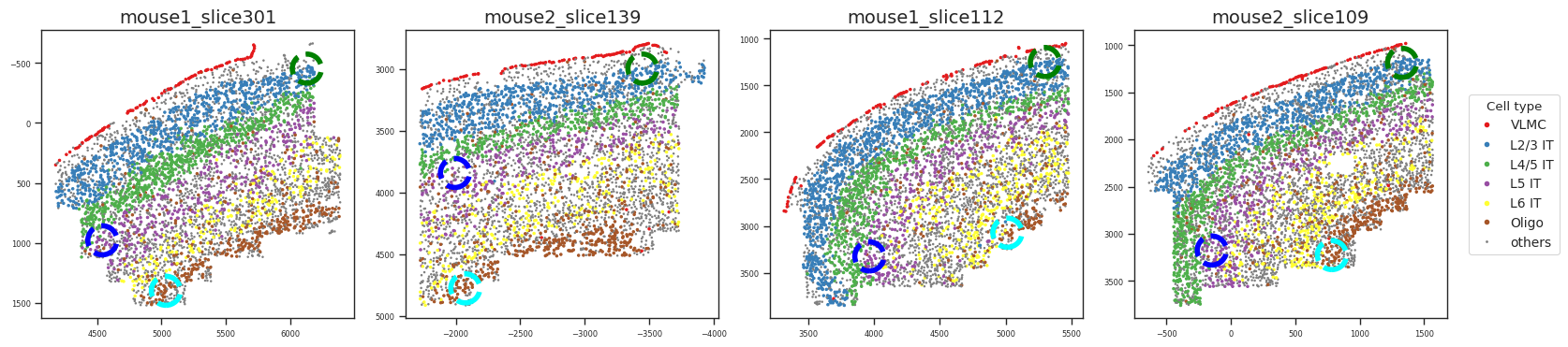
The four slices from different mice exhibit similar structures. We selected three cells from each slice that share a similar microenvironment (cell type composition).

Spatial NT Score Distribution of Selected Samples

data_df = ana_data.meta_data_df.loc[ana_data.meta_data_df['Sample'].isin(selected_samples)].join(ana_data.NT_score[['Cell_NTScore']])  # selected samples for visualization
plot_data_df = data_df.copy()
plot_data_df.loc[plot_data_df['Sample']=='mouse2_slice139','x'] = data_df.loc[plot_data_df['Sample']=='mouse2_slice139','y']
plot_data_df.loc[plot_data_df['Sample']=='mouse2_slice139','y'] = data_df.loc[plot_data_df['Sample']=='mouse2_slice139','x']
plot_data_df.loc[:,'color'] = 1 - plot_data_df['Cell_NTScore'] if options.reverse else plot_data_df['Cell_NTScore']
plot_data_df.head()

	Sample	Cell_Type	x	y	Embedding_1	Embedding_2	Cell_NTScore	color
Cell_ID
100006878605830627922364612565348097824	mouse2_slice109	SMC	805.848948	1215.458623	8.902917	11.969505	0.996727	0.003273
100048801985494957069277355580243213453	mouse1_slice112	Astro	3729.231400	3758.088746	1.808534	8.124959	0.776955	0.223045
10005934872894141098004245916130294941	mouse1_slice112	Endo	4497.223901	2174.526495	6.205052	9.715218	0.436736	0.563264
100067895848056932461806120622152951315	mouse2_slice109	Micro	-298.459511	3240.207594	7.163212	5.260627	0.579384	0.420616
100081856573013143402587078828340349285	mouse2_slice139	Astro	-3127.453806	3438.259872	3.144731	8.946029	0.554079	0.445921

with sns.axes_style('white', rc={
        'xtick.bottom': True,
        'ytick.left': True
}), sns.plotting_context('paper',
                         rc={
                             'axes.titlesize': 14,
                             'axes.labelsize': 8,
                             'xtick.labelsize': 6,
                             'ytick.labelsize': 6,
                             'legend.fontsize': 10
                         }):
    fig = plt.figure(figsize=(20.5, 4))
    axes = []
    gs = gridspec.GridSpec(nrows=1, ncols=5, width_ratios=[5,5,5,5,.5])
    
    # samples
    for index, sample in enumerate(selected_samples):
        sample_data_df = plot_data_df[plot_data_df['Sample']==sample]
        axes.append(fig.add_subplot(gs[index]))
        axes[index].scatter(sample_data_df['x'],
                            sample_data_df['y'],
                            c=sample_data_df['color'],
                            cmap='rainbow',
                            vmin=0,
                            vmax=1,
                            s=2,)
        axes[index].scatter(
            plot_data_df.loc[seletec_cells[index]]['x'],
            plot_data_df.loc[seletec_cells[index]]['y'],
            c='None',
            edgecolors=selected_cell_colors,
            linewidths=4,
            linestyle='--',
            s=500,
        )
        axes[index].set_title(sample)
        
    axes[0].invert_yaxis()
    axes[1].invert_xaxis()
    axes[1].invert_yaxis()
    axes[2].invert_yaxis()
    axes[3].invert_yaxis()
    
    # legend
    axes.append(fig.add_subplot(gs[-1]))
    gradient = np.linspace(1, 0, 1000).reshape(-1, 1)
    axes[-1].imshow(gradient, aspect='auto', cmap='rainbow')
    axes[-1].set_xticks([])
    axes[-1].set_yticks(np.linspace(0, 1000, 6))
    axes[-1].set_yticklabels([f'{x:.01f}' for x in np.linspace(0, 1, 6)])
    axes[-1].set_ylabel('Cell-level NT Score')
    
    fig.savefig('Multisamples_spatial_NTScore.pdf', transparent=True)
    fig.savefig('Multisamples_spatial_NTScore.png', dpi=300)

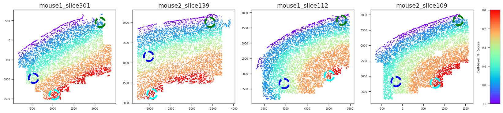
ONTraC generates consistent spatial trajectories (NT score) across multiple slices.

Cell Type Composition of Niches Anchored to Selected Cells

fig, axes = plt.subplots(1, 3, figsize=(12, 4))
for i in range(3):
    
    raw_ctc_df = ana_data.cell_type_composition.loc[seletec_cells[:,i]]
    
    selected_ctc_df = raw_ctc_df[raw_ctc_df.sum().sort_values(ascending=False)[:5].index]
    selected_ctc_df.loc[:,'Sample'] = selected_samples

    plot_data_df = selected_ctc_df.melt(id_vars=['Sample'],value_vars=selected_ctc_df.columns.tolist()[:5], var_name='Cell Type', value_name='Cell Type Composition',ignore_index=True)
    
    sns.barplot(data=plot_data_df,
                x='Sample',
                y='Cell Type Composition',
                hue='Cell Type',
                ax=axes[i])
    axes[i].legend(loc='upper left', bbox_to_anchor=(1,1), title='Cell Type')
    axes[i].set_xticklabels(axes[i].get_xticklabels(), rotation=45)
    axes[i].set_title(f'Selected Cells {i+1}', c=selected_cell_colors[i])
    
fig.tight_layout()
fig.savefig('Multisamples_cell_type_composition_of_selected_cells.pdf', transparent=True)
fig.savefig('Multisamples_cell_type_composition_of_selected_cells.png', dpi=300)

/tmp/ipykernel_836317/3960292759.py:7: SettingWithCopyWarning: 
A value is trying to be set on a copy of a slice from a DataFrame.
Try using .loc[row_indexer,col_indexer] = value instead

See the caveats in the documentation: https://pandas.pydata.org/pandas-docs/stable/user_guide/indexing.html#returning-a-view-versus-a-copy
  selected_ctc_df.loc[:,'Sample'] = selected_samples
/tmp/ipykernel_836317/3960292759.py:17: UserWarning: set_ticklabels() should only be used with a fixed number of ticks, i.e. after set_ticks() or using a FixedLocator.
  axes[i].set_xticklabels(axes[i].get_xticklabels(), rotation=45)
/tmp/ipykernel_836317/3960292759.py:7: SettingWithCopyWarning: 
A value is trying to be set on a copy of a slice from a DataFrame.
Try using .loc[row_indexer,col_indexer] = value instead

See the caveats in the documentation: https://pandas.pydata.org/pandas-docs/stable/user_guide/indexing.html#returning-a-view-versus-a-copy
  selected_ctc_df.loc[:,'Sample'] = selected_samples
/tmp/ipykernel_836317/3960292759.py:17: UserWarning: set_ticklabels() should only be used with a fixed number of ticks, i.e. after set_ticks() or using a FixedLocator.
  axes[i].set_xticklabels(axes[i].get_xticklabels(), rotation=45)
/tmp/ipykernel_836317/3960292759.py:7: SettingWithCopyWarning: 
A value is trying to be set on a copy of a slice from a DataFrame.
Try using .loc[row_indexer,col_indexer] = value instead

See the caveats in the documentation: https://pandas.pydata.org/pandas-docs/stable/user_guide/indexing.html#returning-a-view-versus-a-copy
  selected_ctc_df.loc[:,'Sample'] = selected_samples
/tmp/ipykernel_836317/3960292759.py:17: UserWarning: set_ticklabels() should only be used with a fixed number of ticks, i.e. after set_ticks() or using a FixedLocator.
  axes[i].set_xticklabels(axes[i].get_xticklabels(), rotation=45)

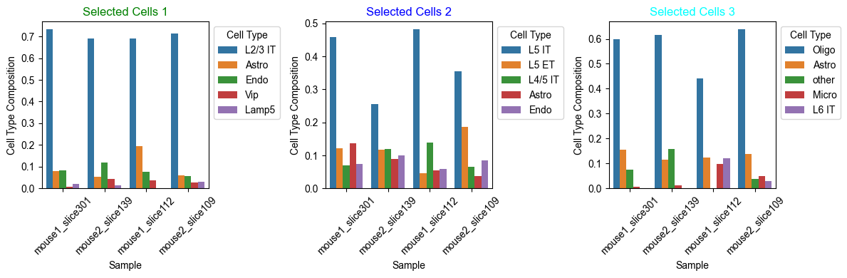
Niches anchored to seletec cells exhibit similar cell type compositions.

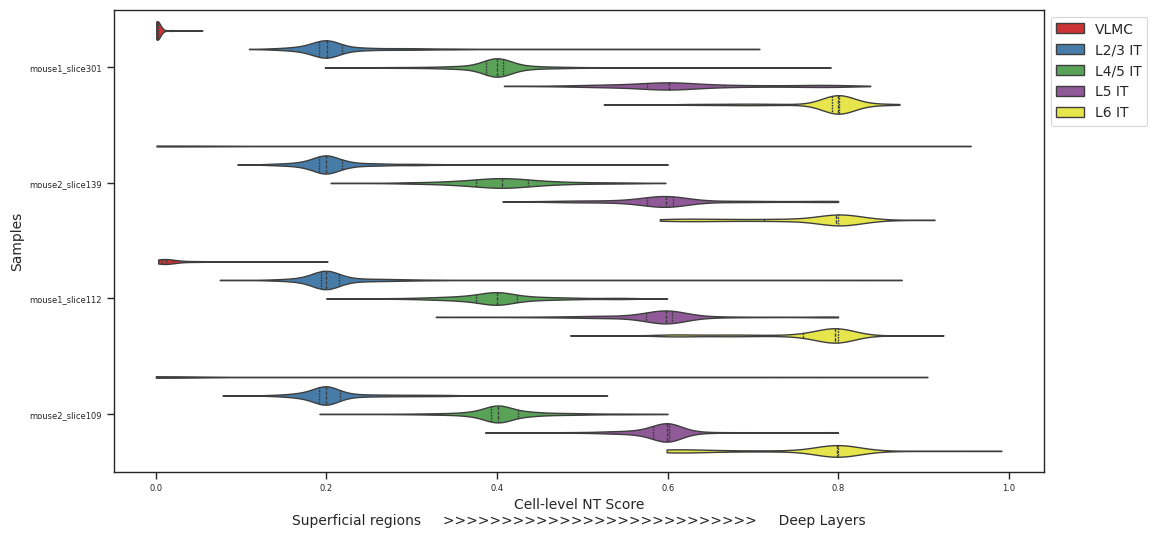
Spatially Localized Cell Types Share Similar NT Scores across Samples

data_df = ana_data.meta_data_df.join(ana_data.NT_score[['Cell_NTScore']]).join(raw_meta_data[['cortical_depth']])
data_df.loc[:,'Cell_NTScore'] = 1 - data_df['Cell_NTScore'] if options.reverse else data_df['Cell_NTScore']
data_df.loc[:,'norm_cortical_depth'] = data_df.loc[:,'cortical_depth'].values / data_df.loc[:,'cortical_depth'].values.max()
data_df.head()

	Sample	Cell_Type	x	y	Embedding_1	Embedding_2	Cell_NTScore	cortical_depth	norm_cortical_depth
Cell_ID
10000143038275111136124942858811168393	mouse2_slice31	Astro	4738.402723	3075.604074	2.155048	7.127876	0.601854	888.114748	0.374428
100001798412490480358118871918100400402	mouse2_slice160	Endo	-3965.470904	1451.943297	5.790349	11.770921	0.771806	1449.123485	0.610949
100006878605830627922364612565348097824	mouse2_slice109	SMC	805.848948	1215.458623	8.902917	11.969505	0.003273	22.943763	0.009673
100007228202835962319771548915451072492	mouse1_slice71	Endo	1347.655448	-3589.803355	5.535499	12.307374	0.785716	1086.621925	0.458118
100009332472089331948140672873134747603	mouse2_slice219	L2/3 IT	-3584.216904	-1883.214455	0.248998	16.258825	0.200618	308.178627	0.129928

selected_cell_types_ = selected_cell_types[:]
selected_cell_types_.remove('Oligo')
plot_data_df = data_df[(data_df['Sample'].isin(selected_samples)) & (data_df['Cell_Type'].isin(selected_cell_types_))][['Sample','Cell_Type','Cell_NTScore']]
plot_data_df['Sample'] = pd.Categorical(plot_data_df['Sample'], categories=selected_samples)  # remove unused samples
plot_data_df['Cell_Type'] = pd.Categorical(plot_data_df['Cell_Type'], categories=selected_cell_types_)  # remove unused cell types
plot_data_df.head()

	Sample	Cell_Type	Cell_NTScore
Cell_ID
100106378211286780818879112257146169937	mouse1_slice112	L2/3 IT	0.199834
10013848917901580372984707123288841246	mouse1_slice301	L2/3 IT	0.306513
100160195205774348243612139282662971606	mouse1_slice112	L4/5 IT	0.459411
100179412288981831083890706042055546088	mouse1_slice112	L4/5 IT	0.334687
100203393073383662058607743517170536086	mouse1_slice301	L4/5 IT	0.378311

with sns.axes_style('white', rc={
        'xtick.bottom': True,
        'ytick.left': True
}), sns.plotting_context('paper',
                         rc={
                             'axes.titlesize': 14,
                             'axes.labelsize': 10,
                             'xtick.labelsize': 6,
                             'ytick.labelsize': 6,
                             'legend.fontsize': 10
                         }):
    fig, ax = plt.subplots(figsize=(12, 6))
    sns.violinplot(
        data=plot_data_df,
        x='Cell_NTScore',
        y='Sample',
        hue='Cell_Type',
        palette=my_pal,
        inner='quart',
        cut=0,
        ax=ax
    )
    ax.legend(loc='upper left', bbox_to_anchor=(1,1))
    ax.set_xlabel('Cell-level NT Score\nSuperficial regions     >>>>>>>>>>>>>>>>>>>>>>>>>>>     Deep Layers')
    ax.set_ylabel('Samples')
    fig.savefig('Multisamples_violin_selected_ct_in_selected_samples_Cell_NTScore.pdf', transparent=True)
    fig.savefig('Multisamples_violin_selected_ct_in_selected_samples_Cell_NTScore.png', dpi=300)

Session Info

session_info.show()

Click to view session information

-----
ONTraC              1.2.2
matplotlib          3.8.4
numpy               1.26.4
pandas              2.2.1
requests            2.31.0
scipy               1.14.1
seaborn             0.13.2
session_info        1.0.0
-----

Click to view modules imported as dependencies

PIL                 10.3.0
asttokens           NA
certifi             2024.02.02
charset_normalizer  3.3.2
colorama            0.4.6
comm                0.2.2
cycler              0.12.1
cython_runtime      NA
dateutil            2.9.0.post0
debugpy             1.8.1
decorator           5.1.1
executing           2.0.1
fontTools           4.51.0
idna                3.7
ipykernel           6.29.4
jedi                0.19.1
kiwisolver          1.4.5
matplotlib_inline   0.1.7
mpl_toolkits        NA
packaging           24.0
parso               0.8.4
patsy               0.5.6
platformdirs        4.2.1
prompt_toolkit      3.0.43
psutil              5.9.8
pure_eval           0.2.2
pydev_ipython       NA
pydevconsole        NA
pydevd              2.9.5
pydevd_file_utils   NA
pydevd_plugins      NA
pydevd_tracing      NA
pygments            2.17.2
pyparsing           3.1.2
pytz                2024.1
six                 1.16.0
stack_data          0.6.3
statsmodels         0.14.4
tornado             6.4
traitlets           5.14.3
typing_extensions   NA
urllib3             2.2.1
wcwidth             0.2.13
yaml                6.0.1
zmq                 26.0.2

-----
IPython             8.23.0
jupyter_client      8.6.1
jupyter_core        5.7.2
-----
Python 3.11.9 | packaged by conda-forge | (main, Apr 19 2024, 18:36:13) [GCC 12.3.0]
Linux-5.14.0-427.13.1.el9_4.x86_64-x86_64-with-glibc2.34
-----
Session information updated at 2025-08-17 23:24