Running ONTraC on MERFISH dataset

Notes

This notebook will show you the process of running ONTraC on simulation data.

We assume that you have installed ONTraC according to the installation tutorial and open this notebook using installed Python kernel (Python 3.11 (ONTraC)).

Running ONTraC on MERFISH data

If your default shell is not Bash, please adjust this code.

ONTraC will run on CPU if CUDA is not available.

Warning: The MERFISH dataset is quite large and will take a long time to run on CPU only.

Download merfish_dataset.csv from Zenodo

%%bash

source ~/.bash_profile
conda activate ONTraC
ONTraC --meta-input original_data.csv --NN-dir merfish_NN --GNN-dir merfish_GNN --NT-dir merfish_NT --device cuda --epochs 1000 --batch-size 10 -s 42 --lr 0.03 --hidden-feats 4 -k 6 --modularity-loss-weight 0.3 --regularization-loss-weight 0.1 --purity-loss-weight 300 --beta 0.03 > log/merfish.log

Results visualization

Please see post analysis tutorial for details.

Install required packages

If you default sh is not bash, please adjust this code

%%bash

source ~/.bash_profile
conda activate ONTraC

pip install ONTraC[analysis]

Loading results

from ONTraC.analysis.data import AnaData
from optparse import Values

options = Values()
options.NN_dir = 'simulation_NN'
options.GNN_dir = 'simulation_GNN'
options.NT_dir = 'simulation_NT'
options.log = 'simulation.log'
options.reverse = True  # Set it to False if you don't want reverse NT score
options.output = None  # We save the output figure by our self here
ana_data = AnaData(options)

Plotting prepare

import numpy as np
import pandas as pd

import matplotlib as mpl

mpl.rcParams['pdf.fonttype'] = 42
mpl.rcParams['ps.fonttype'] = 42
mpl.rcParams['font.family'] = 'Arial'
import matplotlib.pyplot as plt
import seaborn as sns

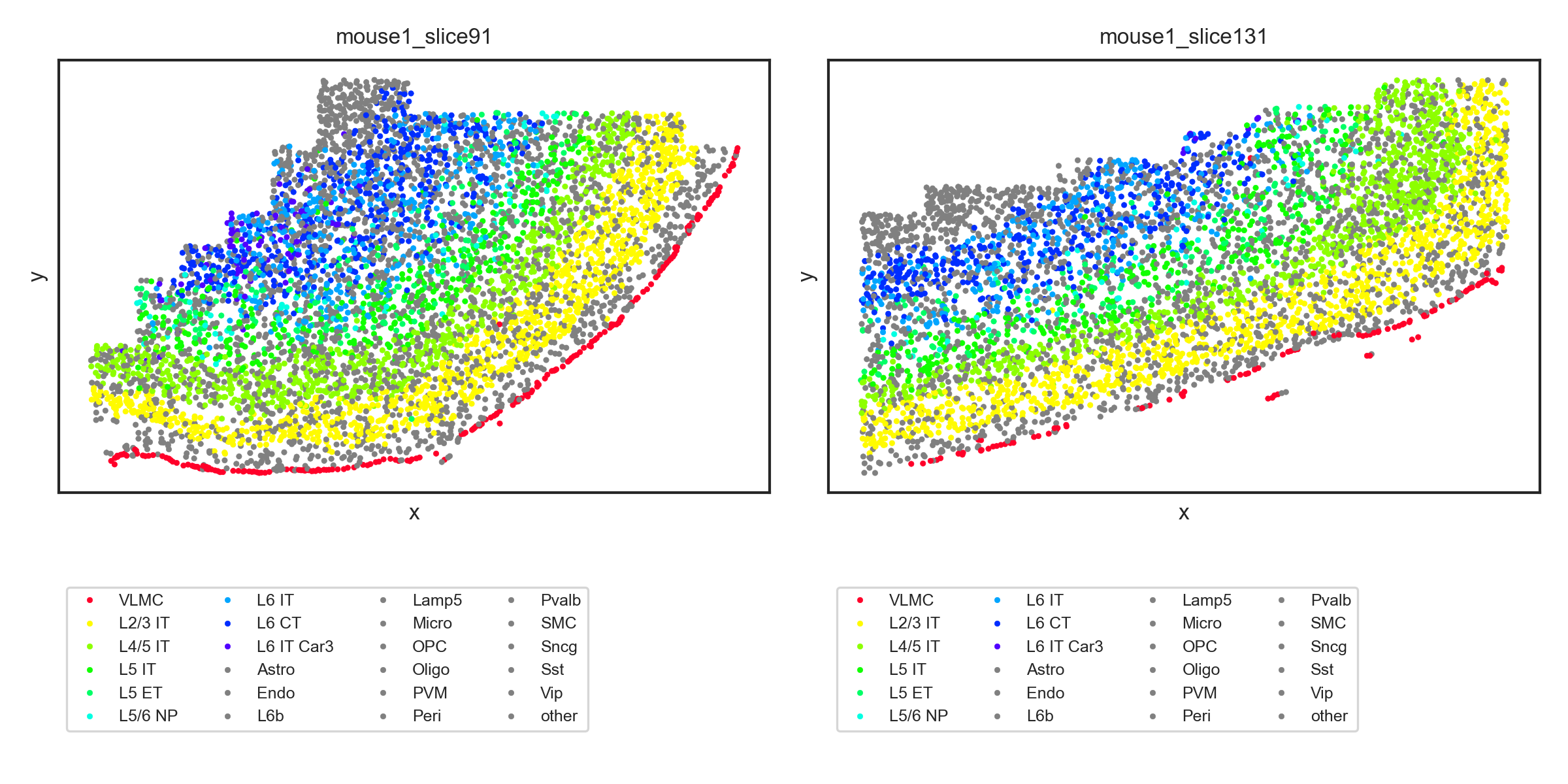
Spatial cell type distribution

cell_types = ana_data.cell_type_codes['Cell_Type'].tolist()
selected_cell_types = ["VLMC", 'L2/3 IT', 'L4/5 IT', 'L5 IT',"L5 ET", "L5/6 NP" , 'L6 IT',"L6 CT","L6 IT Car3"]

rainbow_cmap = mpl.colormaps['gist_rainbow']

my_pal = {"VLMC": rainbow_cmap(0)}
my_pal.update({cell_type: rainbow_cmap( 0.3 + 0.7 * (i - 1) / (len(selected_cell_types) - 1)) for i, cell_type in enumerate(selected_cell_types[1:])})
my_pal.update({cell_type: 'gray' for cell_type in cell_types if cell_type not in selected_cell_types})

# we only show two samples here

seleted_samples = ['mouse1_slice91', 'mouse1_slice131']

data_df = ana_data.meta_data_df[[x in seleted_samples for x in ana_data.meta_data_df['Sample']]]

with sns.axes_style('white', rc={
        'xtick.bottom': True,
        'ytick.left': True
}), sns.plotting_context('paper',
                         rc={
                             'axes.titlesize': 8,
                             'axes.labelsize': 8,
                             'xtick.labelsize': 6,
                             'ytick.labelsize': 6,
                             'legend.fontsize': 6
                         }):
    N = len(seleted_samples)
    fig, axes = plt.subplots(1, N, figsize = (4 * N, 4))
    for i, sample in enumerate(seleted_samples):
        sample_df = data_df.loc[data_df['Sample'] == sample]
        ax = axes[i] if N > 1 else axes
        sns.scatterplot(data = sample_df,
                        x = 'x',
                        y = 'y',
                        hue = 'Cell_Type',
                        palette = my_pal,
                        hue_order = selected_cell_types + [x for x in cell_types if x not in selected_cell_types],
                        edgecolor=None,
                        s = 4,
                        ax=ax)
        ax.set_xticks([])
        ax.set_yticks([])
        ax.set_title(f"{sample}")
        ax.legend(loc='upper left', bbox_to_anchor=(0,-0.2), ncol=4)


    fig.tight_layout()
    fig.savefig('figures/spatial_cell_type.png', dpi=300)

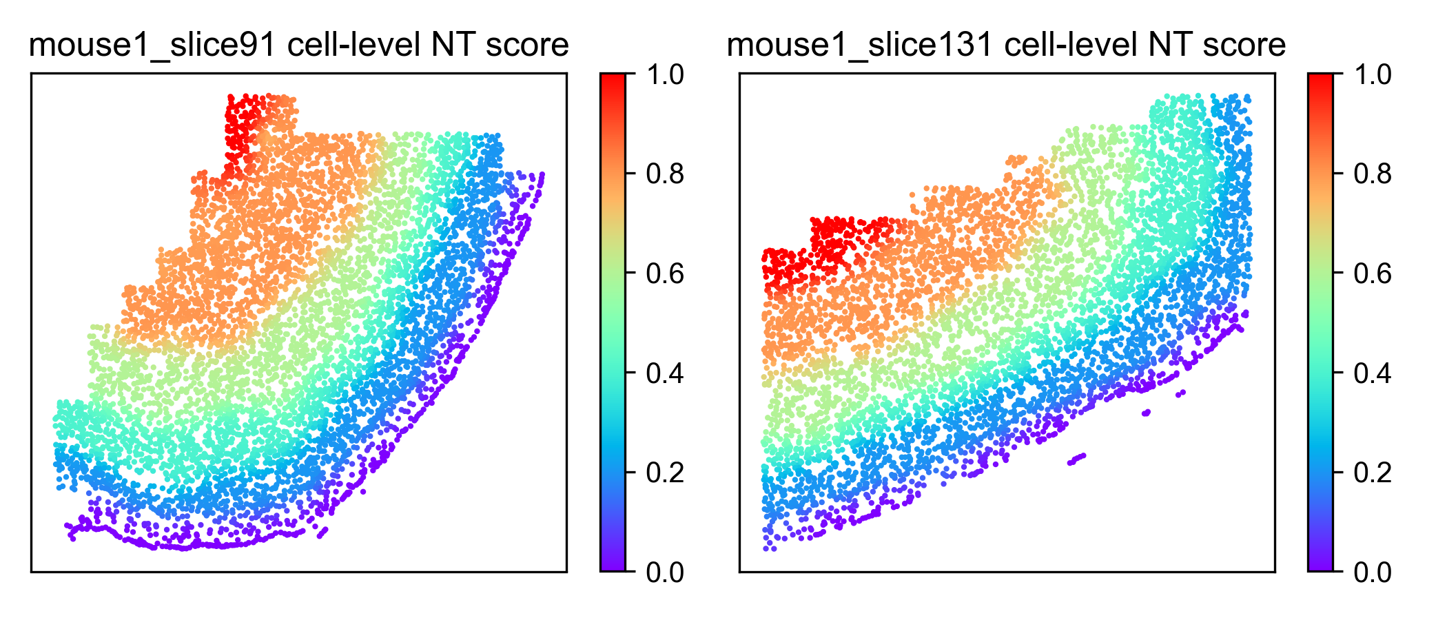
Cell-level NT score spatial distribution

N = len(seleted_samples)
fig, axes = plt.subplots(1, N, figsize = (3.5 * N, 3))
for i, sample in enumerate(seleted_samples):
    sample_df = data_df.loc[data_df['Sample'] == sample]
    sample_df = sample_df.join(ana_data.NT_score['Cell_NTScore'])
    ax = axes[i] if N > 1 else axes
    scatter = ax.scatter(sample_df['x'], sample_df['y'], c=1 - sample_df['Cell_NTScore'], cmap='rainbow', vmin=0, vmax=1, s=1) # substitute with following line if you don't need change the direction of NT score
    # scatter = ax.scatter(sample_df['x'], sample_df['y'], c=sample_df['Cell_NTScore'], cmap='rainbow', vmin=0, vmax=1, s=1)
    ax.set_xticks([])
    ax.set_yticks([])
    plt.colorbar(scatter)
    ax.set_title(f"{sample} cell-level NT score")


fig.tight_layout()
fig.savefig('figures/cell_level_NT_score.png', dpi=300)