Spatial trajectory-based analysis tutorial
This tutorial demonstrates how to analyze feature changes along the trajectory inferred by ONTraC. Features may include cell type composition, gene expression, regulon activity, or any other cell-level or niche-level scores.
Load Modules
import numpy as np
import pandas as pd
import matplotlib as mpl
mpl.rcParams['pdf.fonttype'] = 42
mpl.rcParams['ps.fonttype'] = 42
mpl.rcParams['font.sans-serif'] = 'Arial'
import matplotlib.pyplot as plt
import seaborn as sns
from pprint import pprint
%matplotlib inline
from optparse import Values
from ONTraC.analysis.data import AnaData
from ONTraC.utils import write_version_info

write_version_info()
##################################################################################

         ▄▄█▀▀██   ▀█▄   ▀█▀ █▀▀██▀▀█                   ▄▄█▀▀▀▄█
        ▄█▀    ██   █▀█   █     ██    ▄▄▄ ▄▄   ▄▄▄▄   ▄█▀     ▀
        ██      ██  █ ▀█▄ █     ██     ██▀ ▀▀ ▀▀ ▄██  ██
        ▀█▄     ██  █   ███     ██     ██     ▄█▀ ██  ▀█▄      ▄
         ▀▀█▄▄▄█▀  ▄█▄   ▀█    ▄██▄   ▄██▄    ▀█▄▄▀█▀  ▀▀█▄▄▄▄▀

                        version: 1.2.1

##################################################################################
from ONTraC.analysis.trajectory import (construct_meta_cell_along_trajectory,
                                        cal_features_correlation_along_trajectory,
                                        plot_scatter_feat_along_trajectory,
                                        plot_cell_type_composition_along_trajectory_from_anadata,
                                        plot_cell_type_composition_along_trajectory)
Load Data
Download dataset
import requests

# URL of the file
url = "https://zenodo.org/records/15571644/files/Stereo_seq_data.zip"

# Local file path to save the file
file_path = "./Stereo_seq_data.zip"

try:
    # Send a GET request to the URL
    response = requests.get(url)
    response.raise_for_status()  # Check if the request was successful

    # Write the content to the file
    with open(file_path, "wb") as file:
        file.write(response.content)

    print(f"File downloaded and saved to {file_path}")
except requests.exceptions.RequestException as e:
    print(f"An error occurred: {e}")
File downloaded and saved to ./Stereo_seq_data.zip
import zipfile

# Path to the zip file
zip_file_path = "Stereo_seq_data.zip"

# Directory where files will be extracted
extract_to_path = "./"

try:
    # Open the zip file
    with zipfile.ZipFile(zip_file_path, 'r') as zip_ref:
        # Extract all files to the specified directory
        zip_ref.extractall(extract_to_path)

    print(f"Files extracted to '{extract_to_path}'")
except zipfile.BadZipFile:
    print("The file is not a valid zip file.")
Files extracted to './'
ONTraC output
vis_options = Values()
vis_options.NN_dir = './Stereo_seq_data/ONTraC_output/stereo_midbrain_base_NN/'
vis_options.GNN_dir = './Stereo_seq_data/ONTraC_output/stereo_midbrain_base_GNN/'
vis_options.NT_dir = './Stereo_seq_data/ONTraC_output/stereo_midbrain_base_NT/'
vis_options.reverse = True
vis_options.output = None
ana_data = AnaData(vis_options)
ana_data.meta_data_df.head()
| Sample | Cell_Type | x | y | |
|---|---|---|---|---|
| Cell_ID | ||||
| E12_E1S3_100034 | E12_E1S3 | Fibro | 15940.0 | 18584.0 |
| E12_E1S3_100035 | E12_E1S3 | Fibro | 15942.0 | 18623.0 |
| E12_E1S3_100191 | E12_E1S3 | Endo | 15965.0 | 18619.0 |
| E12_E1S3_100256 | E12_E1S3 | Fibro | 15969.0 | 18717.0 |
| E12_E1S3_100264 | E12_E1S3 | Fibro | 15974.0 | 18692.0 |
Differentiation potency
ot_res1 = pd.read_csv('./Stereo_seq_data/source/moscot/E14_E16_1_cm.csv.gz', index_col=0)
temp = pd.read_csv('./Stereo_seq_data/source/moscot/ss0_E14_E1S3_loc.csv.gz',index_col = 0)
ot_res1.index = temp.index
temp = pd.read_csv('./Stereo_seq_data/source/moscot/ss0_E16_E1S3_loc.csv.gz',index_col = 0)
ot_res1.columns = temp.index
ot_res1.iloc[:5,:3]
| E16_E1S3_21 | E16_E1S3_22 | E16_E1S3_23 | |
|---|---|---|---|
| E14_E1S3_170808 | 0.0 | 0.0 | 0.0 |
| E14_E1S3_170916 | 0.0 | 0.0 | 0.0 |
| E14_E1S3_170934 | 0.0 | 0.0 | 0.0 |
| E14_E1S3_171016 | 0.0 | 0.0 | 0.0 |
| E14_E1S3_171024 | 0.0 | 0.0 | 0.0 |
ot_res2 = pd.read_csv('./Stereo_seq_data/source/moscot/E14_E16_2_cm.csv.gz', index_col=0)
temp = pd.read_csv('./Stereo_seq_data/source/moscot/ss0_E14_E1S3_loc.csv.gz',index_col = 0)
ot_res2.index = temp.index
temp = pd.read_csv('./Stereo_seq_data/source/moscot/ss0_E16_E2S6_loc.csv.gz',index_col = 0)
ot_res2.columns = temp.index
ot_res2.iloc[:5,:3]
| E16_E2S6_119 | E16_E2S6_147 | E16_E2S6_164 | |
|---|---|---|---|
| E14_E1S3_170808 | 0.0 | 0.0 | 0.0 |
| E14_E1S3_170916 | 0.0 | 0.0 | 0.0 |
| E14_E1S3_170934 | 0.0 | 0.0 | 0.0 |
| E14_E1S3_171016 | 0.0 | 0.0 | 0.0 |
| E14_E1S3_171024 | 0.0 | 0.0 | 0.0 |
ot_res3 = pd.read_csv('./Stereo_seq_data/source/moscot/E14_E16_3_cm.csv.gz', index_col=0)
temp = pd.read_csv('./Stereo_seq_data/source/moscot/ss0_E14_E1S3_loc.csv.gz',index_col = 0)
ot_res3.index = temp.index
temp = pd.read_csv('./Stereo_seq_data/source/moscot/ss0_E16_E2S7_loc.csv.gz',index_col = 0)
ot_res3.columns = temp.index
ot_res3.iloc[:5,:3]
| E16_E2S7_291152 | E16_E2S7_291165 | E16_E2S7_291300 | |
|---|---|---|---|
| E14_E1S3_170808 | 0.0 | 1.598103e-18 | 0.0 |
| E14_E1S3_170916 | 0.0 | 0.000000e+00 | 0.0 |
| E14_E1S3_170934 | 0.0 | 0.000000e+00 | 0.0 |
| E14_E1S3_171016 | 0.0 | 0.000000e+00 | 0.0 |
| E14_E1S3_171024 | 0.0 | 0.000000e+00 | 0.0 |
Gene expression
E14_RGC_scaled_exp = pd.read_csv('./Stereo_seq_data/source/stereo_seq_E14_RGC_scaled_exp.csv.gz', index_col=0)
E14_RGC_scaled_exp.iloc[:5,:3]
| 0610005C13Rik | 0610006L08Rik | 0610009B22Rik | |
|---|---|---|---|
| Cell_ID | |||
| E14_E1S3_171289 | -0.036511 | -0.008535 | -0.198124 |
| E14_E1S3_171863 | -0.036511 | -0.008535 | -0.198124 |
| E14_E1S3_171967 | -0.036511 | -0.008535 | -0.198124 |
| E14_E1S3_171983 | -0.036511 | -0.008535 | -0.198124 |
| E14_E1S3_172013 | -0.036511 | -0.008535 | -0.198124 |
Regulon activities
regulon_aucell_df = pd.read_csv('./Stereo_seq_data/source/stereo_seq.auc.csv.gz', index_col=0)
regulon_aucell_df.iloc[:5,:5]
| Ahr | Alx1 | Alx3 | Alx4 | Ar | |
|---|---|---|---|---|---|
| Cell | |||||
| E12_E1S3_100034 | 0.0 | 0.014262 | 0.009032 | 0.038966 | 0.0 |
| E12_E1S3_100035 | 0.0 | 0.017741 | 0.017087 | 0.000000 | 0.0 |
| E12_E1S3_100191 | 0.0 | 0.009400 | 0.009933 | 0.026062 | 0.0 |
| E12_E1S3_100256 | 0.0 | 0.017928 | 0.017399 | 0.000000 | 0.0 |
| E12_E1S3_100264 | 0.0 | 0.019671 | 0.019565 | 0.042947 | 0.0 |
Spatial distribution of NT scores
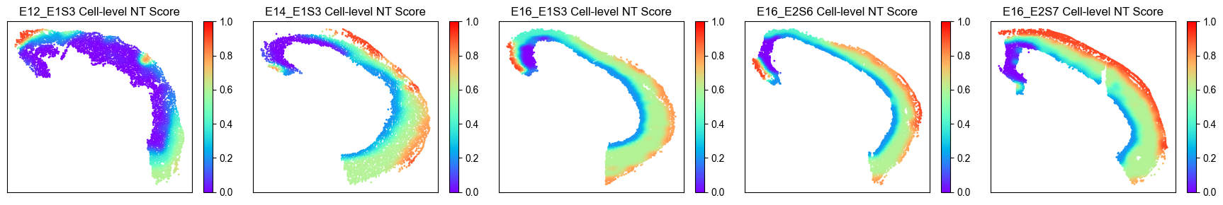
We visualize the spatial distribution of NT scores for each cell to illustrate the spatial trajectory.
Spatial distribution of NT scores for all cells
from ONTraC.analysis.spatial import plot_cell_NT_score_dataset_from_anadata

fig, axes = plot_cell_NT_score_dataset_from_anadata(ana_data)
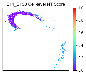
Spatial distribution of NT scores for E14.5 RGCs only
# Selecting E14.5 RGCs from the dataset
plot_meta_data = ana_data.meta_data_df[(ana_data.meta_data_df['Sample'] == 'E14_E1S3') & (ana_data.meta_data_df['Cell_Type'] == 'RGC')]
plot_meta_data.head()
| Sample | Cell_Type | x | y | |
|---|---|---|---|---|
| Cell_ID | ||||
| E14_E1S3_171289 | E14_E1S3 | RGC | 19941.0 | 9116.0 |
| E14_E1S3_171863 | E14_E1S3 | RGC | 20024.0 | 9512.0 |
| E14_E1S3_171967 | E14_E1S3 | RGC | 20040.0 | 9397.0 |
| E14_E1S3_171983 | E14_E1S3 | RGC | 20040.0 | 9219.0 |
| E14_E1S3_172013 | E14_E1S3 | RGC | 20036.0 | 9352.0 |
plot_NT_score = ana_data.NT_score.loc[plot_meta_data.index]
plot_NT_score.head()
| x | y | Niche_NTScore | Cell_NTScore | |
|---|---|---|---|---|
| Cell_ID | ||||
| E14_E1S3_171289 | 19941.0 | 9116.0 | 0.862209 | 0.894205 |
| E14_E1S3_171863 | 20024.0 | 9512.0 | 0.983229 | 0.979535 |
| E14_E1S3_171967 | 20040.0 | 9397.0 | 0.994614 | 0.980553 |
| E14_E1S3_171983 | 20040.0 | 9219.0 | 0.988135 | 0.958657 |
| E14_E1S3_172013 | 20036.0 | 9352.0 | 0.994703 | 0.976718 |
# visualization

from ONTraC.analysis.spatial import plot_cell_NT_score_dataset

fig, ax = plot_cell_NT_score_dataset(meta_data_df=plot_meta_data,
                                     NT_score=plot_NT_score,
                                     reverse=ana_data.options.reverse
                                   )
Cell type composition along spatial trajcetory
Cell type composition along the spatial trajectory reflects changes in the microenvironment.
Cell type composition change for all cells
fig, ax = plot_cell_type_composition_along_trajectory_from_anadata(
    ana_data=ana_data,  # AnaData object
    cell_types=None,  # Column name(s) in AnaData.meta_data_df that contains the cell type information.
                      # Default is None, which means all cell types in AnaData.cell_type_codes will be used.
    agg_cell_num=100,  # Number of cells to aggregate in each bin along the trajectory. Default is 10. 1 means no aggregation.
    figsize=(8,4),  # Figure size. Default is (6, 2).
    palette=None,  # Color palette for cell types. If None, use default color palette. Keys are cell types and values are colors.
    output_file_path=None  # Path to save the figure. If None, the default path
                           # {ana_data.options.output}/lineplot_raw_cell_type_composition_along_trajectory.pdf is used.
                           # If ana_data.options.output is also None, the figure will not be saved and the function
                           # will return the figure and axes objects instead.
)
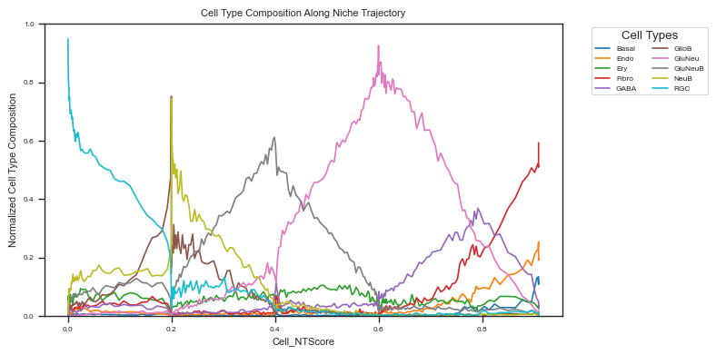
We observe that the dominant cell type shifts along the spatial trajectory, from RGCs (undifferentiated cells) to NeuB, GluNeuB, and ultimately to fully differentiated cells such as GluNeu and GABA neurons.
Cell type composition change for RGC only
# create data_df
data_df = ana_data.meta_data_df.copy()
data_df = data_df.join(1 - ana_data.NT_score['Cell_NTScore'] if hasattr(ana_data.options, 'reverse')
                       and ana_data.options.reverse else ana_data.NT_score['Cell_NTScore'])
data_df = data_df.join(ana_data.cell_type_composition)
# filtering with cell type
data_df = data_df[data_df['Cell_Type'] == 'RGC']
cell_types = ana_data.cell_type_codes['Cell_Type'].values.tolist()
fig ,ax = plot_cell_type_composition_along_trajectory(
    data_df=data_df,
    trajectory='Cell_NTScore',
    cell_types=cell_types, # type: ignore
    agg_cell_num=100,
    figsize=(7,3),
    palette=None,
    output_file_path=None,
)
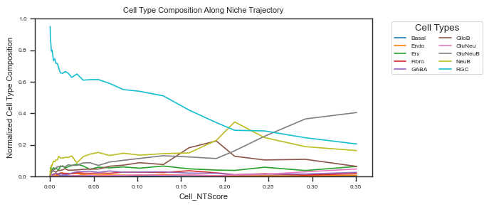
In E14.5, RGCs are primarily located within RGC-dominant microenvironments. Along the spatial trajectory, the proportion of RGCs gradually decreases, while NeuB and GluNeuB cells increase sequentially. We will explore the features associated with this dynamic in the following sections.
Differentiation potency along trajectory
We can investigate differentiation potency by using Moscot to predict the potential offspring of RGCs in the next stage (E16.5). The Moscot output have been loaded in previous section.
Selecting RGCs from Moscot results and aggregate replicates information
target_cells = ana_data.meta_data_df[(ana_data.meta_data_df['Cell_Type'] == 'RGC') & (ana_data.meta_data_df['Sample'] == 'E14_E1S3')]
def ot_res_process(ot_res):
    ot_res = ot_res.loc[ot_res.index.isin(ana_data.meta_data_df.index),
                       ot_res.columns.isin(ana_data.meta_data_df.index)]
    top_5_indices = ot_res.apply(lambda row: row.nlargest(5).index, axis=1)
    top_5_cell_types = top_5_indices.apply(lambda x: ana_data.meta_data_df.loc[x, 'Cell_Type'])
    summary_df = top_5_cell_types.apply(lambda x: x.value_counts(), axis=1).fillna(0).astype(int)
    summary_df = summary_df.loc[target_cells.index]
    summary_df = summary_df.div(summary_df.sum(axis=1).values, axis=0)
    summary_df = summary_df.join(1-ana_data.NT_score['Cell_NTScore'] if hasattr(ana_data.options, 'reverse')
                       and ana_data.options.reverse else ana_data.NT_score['Cell_NTScore'])

    return summary_df
summary_df_1 = ot_res_process(ot_res1)
summary_df_1.iloc[:5,:5]
| Basal | Endo | Ery | Fibro | GABA | |
|---|---|---|---|---|---|
| Cell_ID | |||||
| E14_E1S3_171289 | 0.0 | 0.0 | 0.0 | 0.2 | 0.4 |
| E14_E1S3_171863 | 0.0 | 0.0 | 0.0 | 0.0 | 0.0 |
| E14_E1S3_171967 | 0.0 | 0.0 | 0.0 | 0.0 | 0.0 |
| E14_E1S3_171983 | 0.0 | 0.0 | 0.0 | 0.0 | 0.2 |
| E14_E1S3_172013 | 0.0 | 0.0 | 0.0 | 0.0 | 0.2 |
E14_RGC_metacell_diff_p_1_df = construct_meta_cell_along_trajectory(
    meta_data_df = summary_df_1,
    trajectory = 'Cell_NTScore',
    n_cells = 10)
E14_RGC_metacell_diff_p_1_df.iloc[:5,:5]
| Basal | Endo | Ery | Fibro | GABA | |
|---|---|---|---|---|---|
| Cell_ID | |||||
| E14_E1S3_173789 | 0.0 | 0.0 | 0.00 | 0.00 | 0.02 |
| E14_E1S3_173259 | 0.0 | 0.0 | 0.00 | 0.02 | 0.00 |
| E14_E1S3_174106 | 0.0 | 0.0 | 0.02 | 0.00 | 0.00 |
| E14_E1S3_173417 | 0.0 | 0.0 | 0.00 | 0.02 | 0.08 |
| E14_E1S3_173284 | 0.0 | 0.0 | 0.06 | 0.00 | 0.08 |
summary_df_2 = ot_res_process(ot_res2)
E14_RGC_metacell_diff_p_2_df = construct_meta_cell_along_trajectory(
    meta_data_df = summary_df_2,
    trajectory = 'Cell_NTScore',
    n_cells = 10)
E14_RGC_metacell_diff_p_2_df.iloc[:5,:5]
| Basal | Endo | Ery | Fibro | GABA | |
|---|---|---|---|---|---|
| Cell_ID | |||||
| E14_E1S3_173789 | 0.0 | 0.0 | 0.02 | 0.06 | 0.12 |
| E14_E1S3_173259 | 0.0 | 0.0 | 0.00 | 0.00 | 0.08 |
| E14_E1S3_174106 | 0.0 | 0.0 | 0.02 | 0.04 | 0.04 |
| E14_E1S3_173417 | 0.0 | 0.0 | 0.02 | 0.00 | 0.04 |
| E14_E1S3_173284 | 0.0 | 0.0 | 0.00 | 0.02 | 0.10 |
summary_df_3 = ot_res_process(ot_res3)
E14_RGC_metacell_diff_p_3_df = construct_meta_cell_along_trajectory(
    meta_data_df = summary_df_3,
    trajectory = 'Cell_NTScore',
    n_cells = 10)
E14_RGC_metacell_diff_p_3_df.iloc[:5,:5]
| Basal | Endo | Ery | Fibro | GABA | |
|---|---|---|---|---|---|
| Cell_ID | |||||
| E14_E1S3_173789 | 0.00 | 0.0 | 0.00 | 0.12 | 0.02 |
| E14_E1S3_173259 | 0.02 | 0.0 | 0.02 | 0.04 | 0.02 |
| E14_E1S3_174106 | 0.00 | 0.0 | 0.12 | 0.06 | 0.08 |
| E14_E1S3_173417 | 0.02 | 0.0 | 0.04 | 0.06 | 0.04 |
| E14_E1S3_173284 | 0.00 | 0.0 | 0.02 | 0.06 | 0.12 |
E14_RGC_metacell_diff_p_1_melted_df = E14_RGC_metacell_diff_p_1_df.melt(
    id_vars='Cell_NTScore',
    value_vars=E14_RGC_metacell_diff_p_1_df.columns.tolist()[:-1],
    var_name='Cell type',
    value_name='Proportion')
E14_RGC_metacell_diff_p_1_melted_df['replicate'] = ['rep1'] * E14_RGC_metacell_diff_p_1_melted_df.shape[0]
E14_RGC_metacell_diff_p_1_melted_df.iloc[:5,:5]
| Cell_NTScore | Cell type | Proportion | replicate | |
|---|---|---|---|---|
| 0 | 0.000230 | Basal | 0.0 | rep1 |
| 1 | 0.000240 | Basal | 0.0 | rep1 |
| 2 | 0.000250 | Basal | 0.0 | rep1 |
| 3 | 0.000266 | Basal | 0.0 | rep1 |
| 4 | 0.000285 | Basal | 0.0 | rep1 |
E14_RGC_metacell_diff_p_2_melted_df = E14_RGC_metacell_diff_p_2_df.melt(
    id_vars='Cell_NTScore',
    value_vars=E14_RGC_metacell_diff_p_2_df.columns.tolist()[:-1],
    var_name='Cell type',
    value_name='Proportion')
E14_RGC_metacell_diff_p_2_melted_df['replicate'] = ['rep2'] * E14_RGC_metacell_diff_p_2_melted_df.shape[0]
E14_RGC_metacell_diff_p_2_melted_df.iloc[:5,:5]
| Cell_NTScore | Cell type | Proportion | replicate | |
|---|---|---|---|---|
| 0 | 0.000230 | Basal | 0.0 | rep2 |
| 1 | 0.000240 | Basal | 0.0 | rep2 |
| 2 | 0.000250 | Basal | 0.0 | rep2 |
| 3 | 0.000266 | Basal | 0.0 | rep2 |
| 4 | 0.000285 | Basal | 0.0 | rep2 |
E14_RGC_metacell_diff_p_3_melted_df = E14_RGC_metacell_diff_p_3_df.melt(
    id_vars='Cell_NTScore',
    value_vars=E14_RGC_metacell_diff_p_3_df.columns.tolist()[:-1],
    var_name='Cell type',
    value_name='Proportion')
E14_RGC_metacell_diff_p_3_melted_df['replicate'] = ['rep3'] * E14_RGC_metacell_diff_p_3_melted_df.shape[0]
E14_RGC_metacell_diff_p_3_melted_df.iloc[:5,:5]
| Cell_NTScore | Cell type | Proportion | replicate | |
|---|---|---|---|---|
| 0 | 0.000230 | Basal | 0.00 | rep3 |
| 1 | 0.000240 | Basal | 0.02 | rep3 |
| 2 | 0.000250 | Basal | 0.00 | rep3 |
| 3 | 0.000266 | Basal | 0.02 | rep3 |
| 4 | 0.000285 | Basal | 0.00 | rep3 |
E14_RGC_metacell_diff_p_melted = pd.concat([E14_RGC_metacell_diff_p_1_melted_df,
                                            E14_RGC_metacell_diff_p_2_melted_df,
                                            E14_RGC_metacell_diff_p_3_melted_df])
E14_RGC_metacell_diff_p_melted.head()
| Cell_NTScore | Cell type | Proportion | replicate | |
|---|---|---|---|---|
| 0 | 0.000230 | Basal | 0.0 | rep1 |
| 1 | 0.000240 | Basal | 0.0 | rep1 |
| 2 | 0.000250 | Basal | 0.0 | rep1 |
| 3 | 0.000266 | Basal | 0.0 | rep1 |
| 4 | 0.000285 | Basal | 0.0 | rep1 |
sns.lmplot(data = E14_RGC_metacell_diff_p_melted[E14_RGC_metacell_diff_p_melted['Cell type'].isin(['RGC', 'NeuB'])],
           x = 'Cell_NTScore',
           y = 'Proportion',
           hue = 'Cell type',
           scatter_kws={'edgecolor': None},
           ci=95,
          )
<seaborn.axisgrid.FacetGrid at 0x152d972529d0>
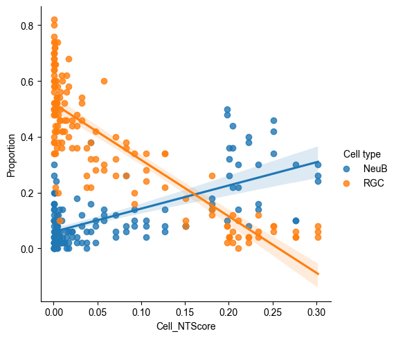
Along the spatial trajectory, the probability of RGCs maintaining their identity decreases, while the probability of their differentiation into NeuB increases.
Gene expression changes along spatial trajectory
Next, we explore gene expression dynamics along the spatial trajectory.
E14_RGC_gene_exp_df = E14_RGC_scaled_exp.join(1 - ana_data.NT_score['Cell_NTScore'] if hasattr(ana_data.options, 'reverse')
                       and ana_data.options.reverse else ana_data.NT_score['Cell_NTScore'])
# The meta-cell could reduce the noise here
E14_RGC_gene_exp_metacell_data_df = construct_meta_cell_along_trajectory(
    meta_data_df = E14_RGC_gene_exp_df,
    trajectory = 'Cell_NTScore',
    n_cells = 10
)
E14_RGC_gene_exp_metacell_data_df.iloc[:5,:3]
| 0610005C13Rik | 0610006L08Rik | 0610009B22Rik | |
|---|---|---|---|
| Cell_ID | |||
| E14_E1S3_173789 | -0.036511 | -0.008535 | -0.198124 |
| E14_E1S3_173259 | -0.036511 | -0.008535 | -0.198124 |
| E14_E1S3_174106 | -0.036511 | -0.008535 | -0.198124 |
| E14_E1S3_173417 | -0.036511 | -0.008535 | -0.198124 |
| E14_E1S3_173284 | -0.036511 | -0.008535 | -0.198124 |
gene_correlated_df = cal_features_correlation_along_trajectory(
    data_df = E14_RGC_gene_exp_metacell_data_df,
    trajectory = 'Cell_NTScore',
    rho_threshold=0.4,
    p_val_threshold=0.01
)
print(gene_correlated_df.shape)
/sc/arion/work/wangw32/conda-env/envs/ONTraC/lib/python3.11/site-packages/ONTraC/analysis/trajectory.py:102: ConstantInputWarning: An input array is constant; the correlation coefficient is not defined.
  rho, p_val = pearsonr(data_df[trajectory], data_df[feat])
(109, 2)
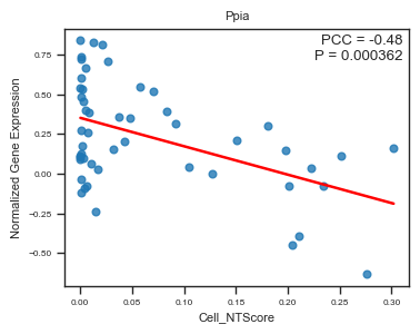
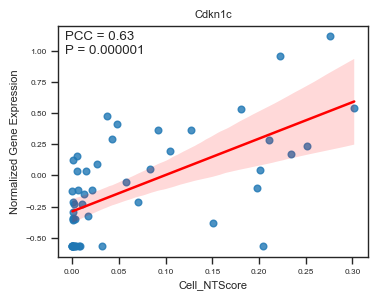
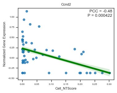
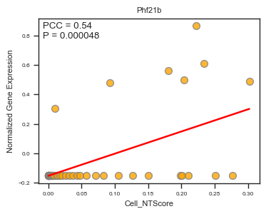
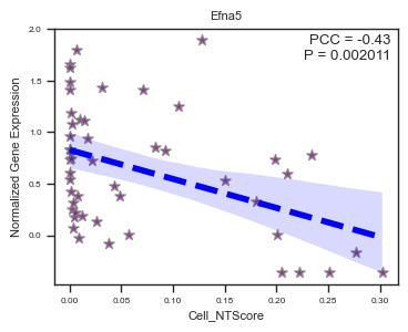
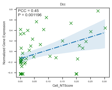
We identified 109 genes whose expression levels are significantly correlated with cell-level NT scores. Here, we highlight six representative genes that are strongly associated with neuronal differentiation and maturation.
gene_correlated_df.head()
| PCC | P_Value | |
|---|---|---|
| Feature | ||
| Cdkn1c | 0.629617 | 9.666948e-07 |
| Gm3764 | 0.623302 | 1.333598e-06 |
| Lbh | 0.618297 | 1.712368e-06 |
| Bbs9 | 0.550067 | 3.502920e-05 |
| Phf21b | 0.542046 | 4.788367e-05 |
fig, ax = plot_scatter_feat_along_trajectory(
    data_df = E14_RGC_gene_exp_metacell_data_df,
    trajectory = 'Cell_NTScore',
    feature = 'Ppia',
    fit_reg = True,
    annotate_pos = 'upper right',
    figszie = (4,3),
    ylabel = 'Normalized Gene Expression',
)
fig, ax = plot_scatter_feat_along_trajectory(
    data_df = E14_RGC_gene_exp_metacell_data_df,
    trajectory = 'Cell_NTScore',
    feature = 'Cdkn1c',
    fit_reg = True,
    annotate_pos = 'upper left',
    figszie = (4,3),
    ylabel = 'Normalized Gene Expression',
    ci=95,  # Size of the confidence interval for the regression estimate
)
fig, ax = plot_scatter_feat_along_trajectory(
    data_df = E14_RGC_gene_exp_metacell_data_df,
    trajectory = 'Cell_NTScore',
    feature = 'Ccnd2',
    fit_reg = True,
    annotate_pos = 'upper right',
    figszie = (4,3),
    ylabel = 'Normalized Gene Expression',
    line_kws = {'color': 'green', 'lw': 4},  # line parameters
    ci=70,  # Size of the confidence interval for the regression estimate
)
fig, ax = plot_scatter_feat_along_trajectory(
    data_df = E14_RGC_gene_exp_metacell_data_df,
    trajectory = 'Cell_NTScore',
    feature = 'Phf21b',
    fit_reg = True,
    annotate_pos = 'upper left',
    figszie = (4,3),
    ylabel = 'Normalized Gene Expression',
    scatter_kws = {'color': 'orange', 'edgecolor': 'gray', 's': 50},  # scatter parameters
)
fig, ax = plot_scatter_feat_along_trajectory(
    data_df = E14_RGC_gene_exp_metacell_data_df,
    trajectory = 'Cell_NTScore',
    feature = 'Efna5',
    fit_reg = True,
    annotate_pos = 'upper right',
    figszie = (4,3),
    ylabel = 'Normalized Gene Expression',
    scatter_kws = {'color': 'purple', 'edgecolor': 'gray', 's': 50},  # scatter parameters
    line_kws = {'color': 'blue', 'lw': 4, 'ls': '--'},  # line parameters
    ci = 95,  # Size of the confidence interval for the regression estimate
    marker = '*',  # Marker to use for the scatterplot glyphs.
)
fig, ax = plot_scatter_feat_along_trajectory(
    data_df = E14_RGC_gene_exp_metacell_data_df,
    trajectory = 'Cell_NTScore',
    feature = 'Dcc',
    fit_reg = True,
    annotate_pos = 'upper left',
    figszie = (4,3),
    ylabel = 'Normalized Gene Expression',
    scatter_kws = {'color': 'green', 's': 50},  # scatter parameters
    line_kws = {'color': 'C0', 'lw': 2, 'ls': '-.'},  # line parameters
    ci = 95,  # Size of the confidence interval for the regression estimate.
    marker = 'x',  # Marker to use for the scatterplot glyphs.
)
You can also select top N genes by following command:
cal_features_correlation_along_trajectory(
    data_df = E14_RGC_gene_exp_metacell_data_df,
    trajectory = 'Cell_NTScore',
    top_n=5,
    rho_threshold=0.4,
    p_val_threshold=0.01
)
/sc/arion/work/wangw32/conda-env/envs/ONTraC/lib/python3.11/site-packages/ONTraC/analysis/trajectory.py:102: ConstantInputWarning: An input array is constant; the correlation coefficient is not defined.
  rho, p_val = pearsonr(data_df[trajectory], data_df[feat])
| PCC | P_Value | |
|---|---|---|
| Feature | ||
| Cdkn1c | 0.629617 | 9.666948e-07 |
| Gm3764 | 0.623302 | 1.333598e-06 |
| Lbh | 0.618297 | 1.712368e-06 |
| Bbs9 | 0.550067 | 3.502920e-05 |
| Phf21b | 0.542046 | 4.788367e-05 |
| Mcm3 | -0.453214 | 9.492690e-04 |
| Eif2s2 | -0.456194 | 8.696506e-04 |
| Tuba1b | -0.470727 | 5.608145e-04 |
| Ccnd2 | -0.479827 | 4.218648e-04 |
| Ppia | -0.484622 | 3.619282e-04 |
Regulon activity changes along spatial trajectory
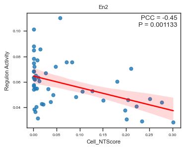
To gain mechanistic insights, we performed gene regulatory network (GRN) analysis using the SCENIC workflow and explore regulon activity changes along spatial trajectory.
E14_RGC_regulon_aucell_df = regulon_aucell_df.loc[target_cells.index]
E14_RGC_regulon_aucell_df = E14_RGC_regulon_aucell_df.join(1-ana_data.NT_score['Cell_NTScore'] if hasattr(ana_data.options, 'reverse')
                       and ana_data.options.reverse else ana_data.NT_score['Cell_NTScore'])
E14_RGC_regulon_aucell_df.iloc[:5,:3]
| Ahr | Alx1 | Alx3 | |
|---|---|---|---|
| Cell_ID | |||
| E14_E1S3_171289 | 0.0 | 0.015500 | 0.014530 |
| E14_E1S3_171863 | 0.0 | 0.018301 | 0.017757 |
| E14_E1S3_171967 | 0.0 | 0.011018 | 0.009434 |
| E14_E1S3_171983 | 0.0 | 0.020709 | 0.000000 |
| E14_E1S3_172013 | 0.0 | 0.009773 | 0.008186 |
E14_RGC_regulon_aucell_metacell_data_df = construct_meta_cell_along_trajectory(meta_data_df = E14_RGC_regulon_aucell_df,
                                                                trajectory = 'Cell_NTScore',
                                                                n_cells = 10)
E14_RGC_regulon_aucell_metacell_data_df.iloc[:5,:3]
| Ahr | Alx1 | Alx3 | |
|---|---|---|---|
| Cell_ID | |||
| E14_E1S3_173789 | 0.0 | 0.012552 | 0.019366 |
| E14_E1S3_173259 | 0.0 | 0.019238 | 0.021671 |
| E14_E1S3_174106 | 0.0 | 0.010374 | 0.022217 |
| E14_E1S3_173417 | 0.0 | 0.024025 | 0.014273 |
| E14_E1S3_173284 | 0.0 | 0.016657 | 0.011069 |
fig, ax = plot_scatter_feat_along_trajectory(
    data_df = E14_RGC_regulon_aucell_metacell_data_df,
    trajectory = 'Cell_NTScore',
    feature = 'En2',
    fit_reg = True,
    annotate_pos = 'upper right',
    figszie = (4,3),
    ylabel = 'Regulon Activity',
    ci = 95,
)
fig, ax = plot_scatter_feat_along_trajectory(
    data_df = E14_RGC_regulon_aucell_metacell_data_df,
    trajectory = 'Cell_NTScore',
    feature = 'Hes6',
    fit_reg = True,
    annotate_pos = 'upper right',
    figszie = (4,3),
    ylabel = 'Regulon Activity',
    ci = 95,
)
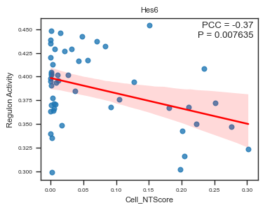
We identified several regulons whose activity scores are significantly correlated with cell-level NT scores (spatial trajectory).
Session Info
import session_info

session_info.show()
Click to view session information
-----
ONTraC              1.2.1
matplotlib          3.8.4
numpy               1.26.4
pandas              2.2.1
requests            2.31.0
seaborn             0.13.2
session_info        1.0.0
-----
Click to view modules imported as dependencies
PIL                 10.3.0
asttokens           NA
certifi             2024.02.02
charset_normalizer  3.3.2
colorama            0.4.6
comm                0.2.2
cycler              0.12.1
cython_runtime      NA
dateutil            2.9.0.post0
debugpy             1.8.1
decorator           5.1.1
executing           2.0.1
idna                3.7
ipykernel           6.29.4
jedi                0.19.1
kiwisolver          1.4.5
matplotlib_inline   0.1.7
mpl_toolkits        NA
packaging           24.0
parso               0.8.4
patsy               0.5.6
platformdirs        4.2.1
prompt_toolkit      3.0.43
psutil              5.9.8
pure_eval           0.2.2
pydev_ipython       NA
pydevconsole        NA
pydevd              2.9.5
pydevd_file_utils   NA
pydevd_plugins      NA
pydevd_tracing      NA
pygments            2.17.2
pyparsing           3.1.2
pytz                2024.1
scipy               1.14.1
six                 1.16.0
stack_data          0.6.3
statsmodels         0.14.4
tornado             6.4
traitlets           5.14.3
typing_extensions   NA
urllib3             2.2.1
wcwidth             0.2.13
yaml                6.0.1
zmq                 26.0.2
-----
IPython             8.23.0
jupyter_client      8.6.1
jupyter_core        5.7.2
-----
Python 3.11.9 | packaged by conda-forge | (main, Apr 19 2024, 18:36:13) [GCC 12.3.0]
Linux-5.14.0-427.13.1.el9_4.x86_64-x86_64-with-glibc2.34
-----
Session information updated at 2025-06-08 22:02