Running ONTraC on a MERFISH dataset
Download the data
Warning: The MERFISH dataset is quite large and will take a long time to run on CPU only.
Download merfish_dataset.csv from Zenodo
Running ONTraC
If your default shell is not Bash, please adjust this code.
ONTraC will run on CPU if CUDA is not available.
conda activate ONTraC
ONTraC --meta-input original_data.csv \
--NN-dir merfish_NN \
--GNN-dir merfish_GNN \
--NT-dir merfish_NT \
--device cuda --epochs 1000 --batch-size 10 -s 42 --lr 0.03 \
--hidden-feats 4 -k 6 --modularity-loss-weight 0.3 \
--regularization-loss-weight 0.1 --purity-loss-weight 300 \
--beta 0.03 > log/merfish.log
Results visualization
Please see the Visualizations tutorials for details.
Loading results
from ONTraC.analysis.data import AnaData
from optparse import Values

options = Values()
options.NN_dir = 'simulation_NN'
options.GNN_dir = 'simulation_GNN'
options.NT_dir = 'simulation_NT'
options.log = 'simulation.log'
options.reverse = True  # Set it to False if you don't want reverse NT score
options.output = None  # We save the output figure by our self here
ana_data = AnaData(options)
Plotting preparation
import numpy as np
import pandas as pd

import matplotlib as mpl

mpl.rcParams['pdf.fonttype'] = 42
mpl.rcParams['ps.fonttype'] = 42
mpl.rcParams['font.family'] = 'Arial'
import matplotlib.pyplot as plt
import seaborn as sns
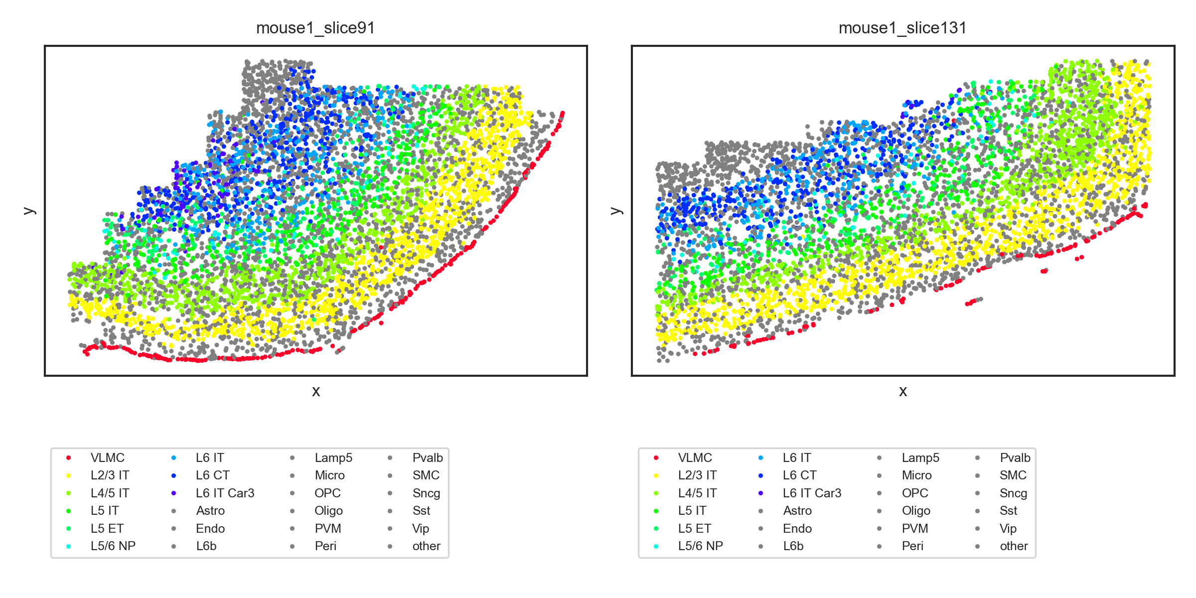
Spatial cell type distribution
cell_types = ana_data.cell_type_codes['Cell_Type'].tolist()
selected_cell_types = ["VLMC", 'L2/3 IT', 'L4/5 IT', 'L5 IT',"L5 ET", "L5/6 NP" , 'L6 IT',"L6 CT","L6 IT Car3"]

rainbow_cmap = mpl.colormaps['gist_rainbow']

my_pal = {"VLMC": rainbow_cmap(0)}
my_pal.update({cell_type: rainbow_cmap( 0.3 + 0.7 * (i - 1) / (len(selected_cell_types) - 1)) for i, cell_type in enumerate(selected_cell_types[1:])})
my_pal.update({cell_type: 'gray' for cell_type in cell_types if cell_type not in selected_cell_types})
We only show two samples here
seleted_samples = ['mouse1_slice91', 'mouse1_slice131']

data_df = ana_data.meta_data_df[[x in seleted_samples for x in ana_data.meta_data_df['Sample']]]
with sns.axes_style('white', rc={
      'xtick.bottom': True,
      'ytick.left': True
}), sns.plotting_context('paper',
                        rc={
                           'axes.titlesize': 8,
                           'axes.labelsize': 8,
                           'xtick.labelsize': 6,
                           'ytick.labelsize': 6,
                           'legend.fontsize': 6
                        }):
   N = len(seleted_samples)
   fig, axes = plt.subplots(1, N, figsize = (4 * N, 4))
   for i, sample in enumerate(seleted_samples):
      sample_df = data_df.loc[data_df['Sample'] == sample]
      ax = axes[i] if N > 1 else axes
      sns.scatterplot(data = sample_df,
                        x = 'x',
                        y = 'y',
                        hue = 'Cell_Type',
                        palette = my_pal,
                        hue_order = selected_cell_types + [x for x in cell_types if x not in selected_cell_types],
                        edgecolor=None,
                        s = 4,
                        ax=ax)
      ax.set_xticks([])
      ax.set_yticks([])
      ax.set_title(f"{sample}")
      ax.legend(loc='upper left', bbox_to_anchor=(0,-0.2), ncol=4)


   fig.tight_layout()
   fig.savefig('figures/spatial_cell_type.png', dpi=300)
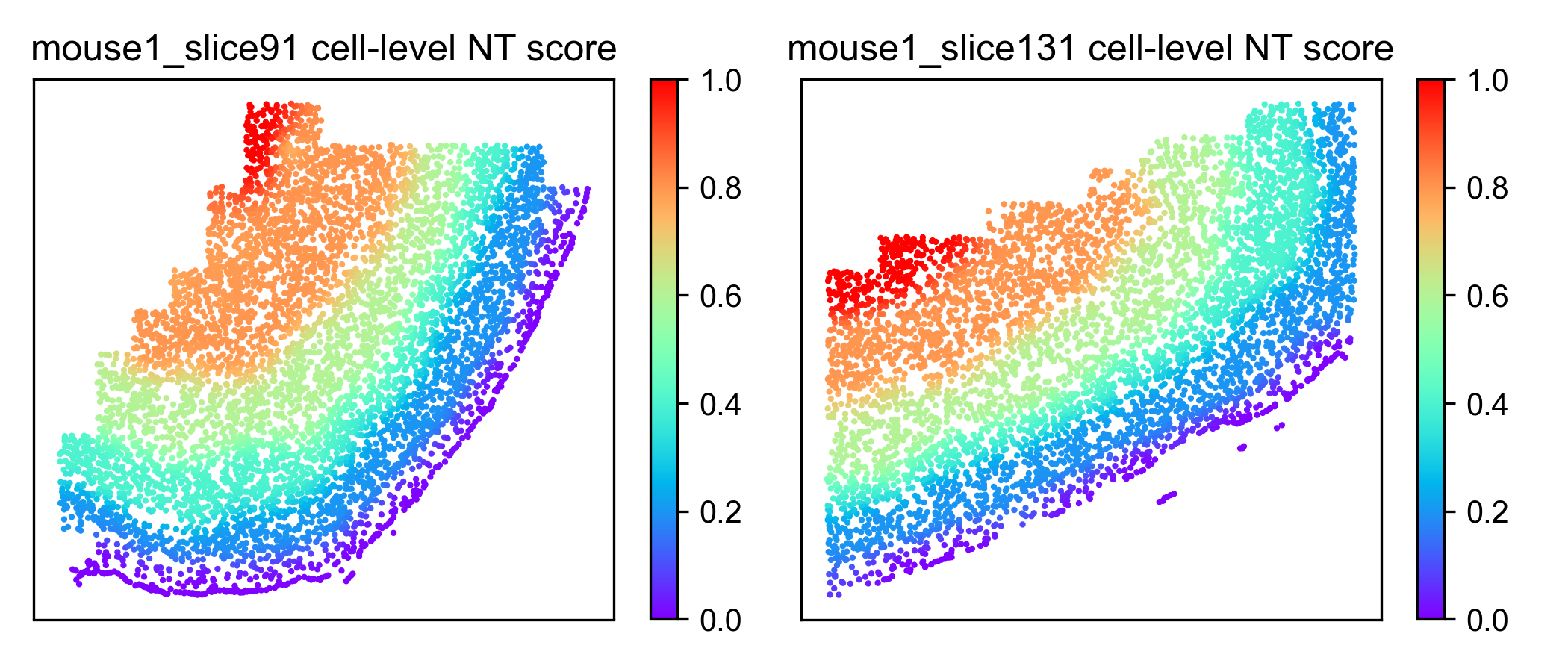
Cell-level NT score spatial distribution
N = len(seleted_samples)
fig, axes = plt.subplots(1, N, figsize = (3.5 * N, 3))
for i, sample in enumerate(seleted_samples):
   sample_df = data_df.loc[data_df['Sample'] == sample]
   sample_df = sample_df.join(ana_data.NT_score['Cell_NTScore'])
   ax = axes[i] if N > 1 else axes
   scatter = ax.scatter(sample_df['x'], sample_df['y'], c=1 - sample_df['Cell_NTScore'], cmap='rainbow', vmin=0, vmax=1, s=1) # substitute with following line if you don't need change the direction of NT score
   # scatter = ax.scatter(sample_df['x'], sample_df['y'], c=sample_df['Cell_NTScore'], cmap='rainbow', vmin=0, vmax=1, s=1)
   ax.set_xticks([])
   ax.set_yticks([])
   plt.colorbar(scatter)
   ax.set_title(f"{sample} cell-level NT score")


fig.tight_layout()
fig.savefig('figures/cell_level_NT_score.png', dpi=300)